Statistical Methods with R

Residuals & Outliers

Unit D · Chapter 10 · Lecture 10b

Developed by Jeffrey M. Girard

Overview

Assumptions Overview

  • Assumptions about the Formula
    • Correct Functional Form
    • Perfectly Measured Predictors
    • No Collinearity/Multicollinearity
  • Assumptions about the Residuals
    • Constant Error Variance
    • Normality of Residuals
    • Independence of Residuals

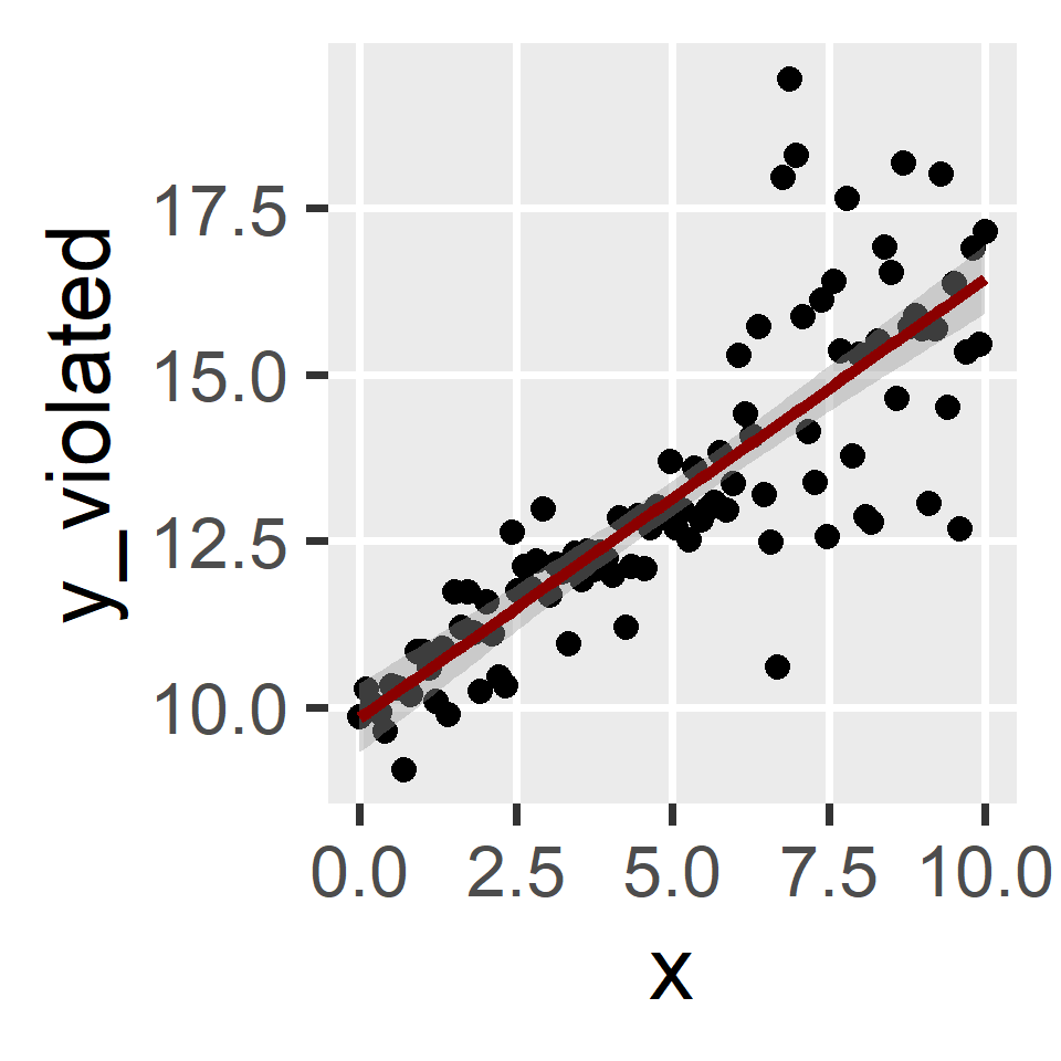
Constant Error Variance

Assumption

  • For any value of \(x\), the residual variance are constant
    • The spread of points around the line must be consistent
    • This is similar to Student’s assumption of equal group variances
  • This is also called “homoscedasticity” or “homogeneity of variance”
    • When violated, we say that there is “heteroscedasticity”

Consequences of Violating

Bias in standard errors only

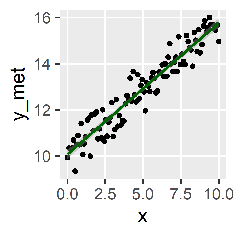
Assumption Examples

Diagnostics

  1. Breusch-Pagan heteroscedasticity test
    • A significant result indicates heteroscedasticity
    • But this test gets more power with a larger sample…

check_heteroscedasticity(fit)

  1. Plot the residuals against the fitted values
    • (Or some derivative of the residuals)

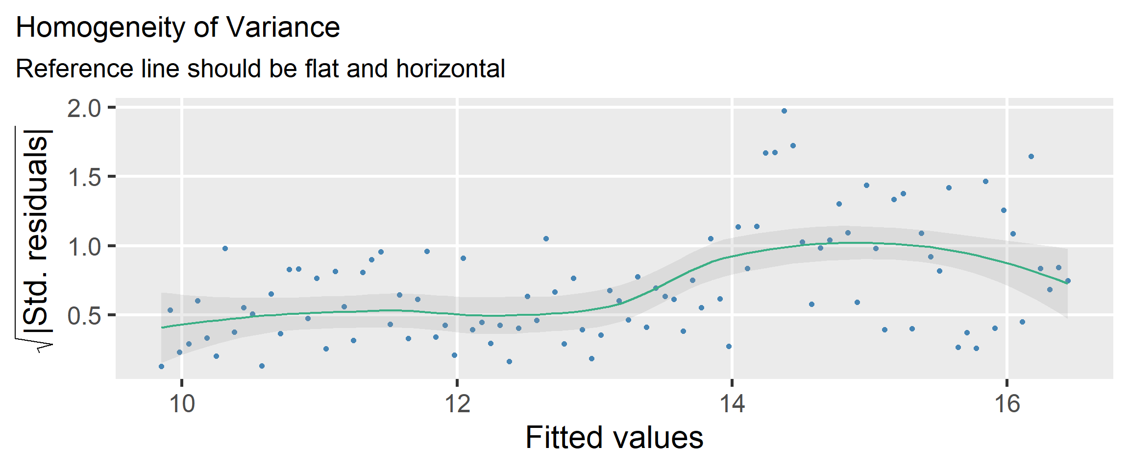
check_model(fit, check = "homogeneity")

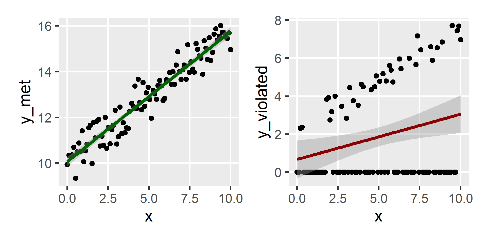
Example: Assumption Met

library(easystats)
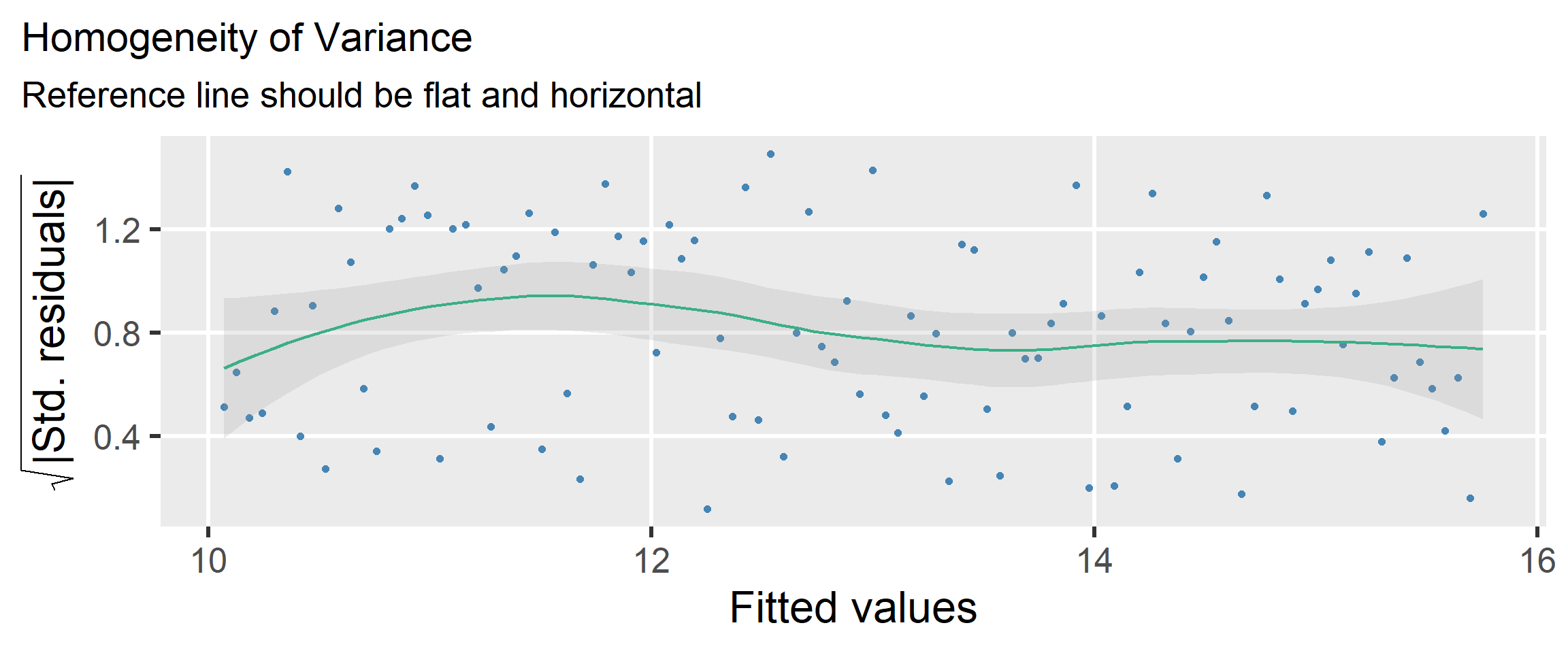
check_heteroscedasticity(fit_met)
## OK: Error variance appears to be homoscedastic (p = 0.192).
check_model(fit_met, check = "homogeneity")
Example: Assumption Violated

check_heteroscedasticity(fit_violated)
## Warning: Heteroscedasticity (non-constant error variance) detected (p < .001).
check_model(fit_violated, check = "homogeneity")
Solutions

  1. Transform the outcome variable
    • e.g., Log or power transformations
  2. Adjust the standard errors
    • e.g., Huber-White (sandwich) estimation
  3. Model the error variance explicitly
    • e.g., weighted least squares estimation
    • e.g., location-scale models

Normal Residuals

Assumption

  • The residuals are normally distributed around the line
    • The spread around the line is a bell curve
    • This is more problematic with smaller samples
    • Non-normal residuals may signal other problems

Consequences of Violating

Standard errors will be biased

Examples

Diagnostics

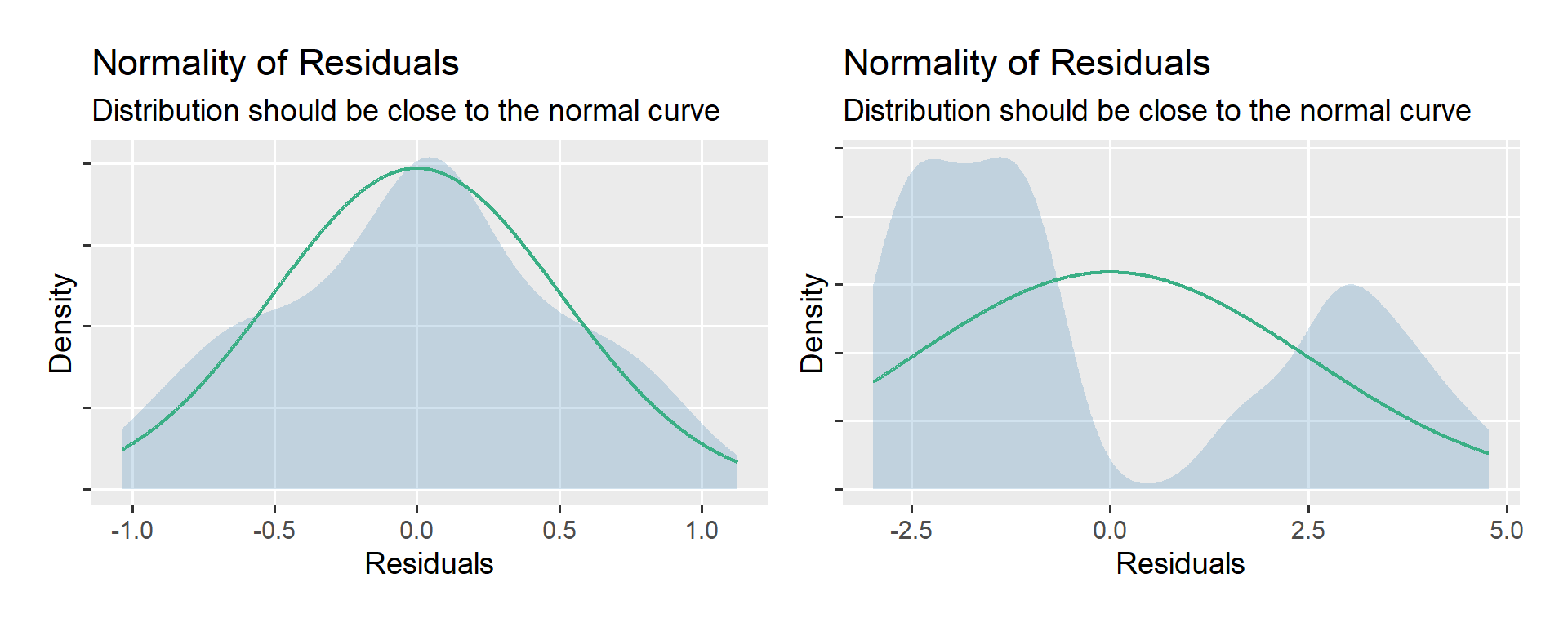
  1. Plot the residuals’ distribution
    • Visually compare density plot to normal distribution
    • Assumption is violated to the extent they differ
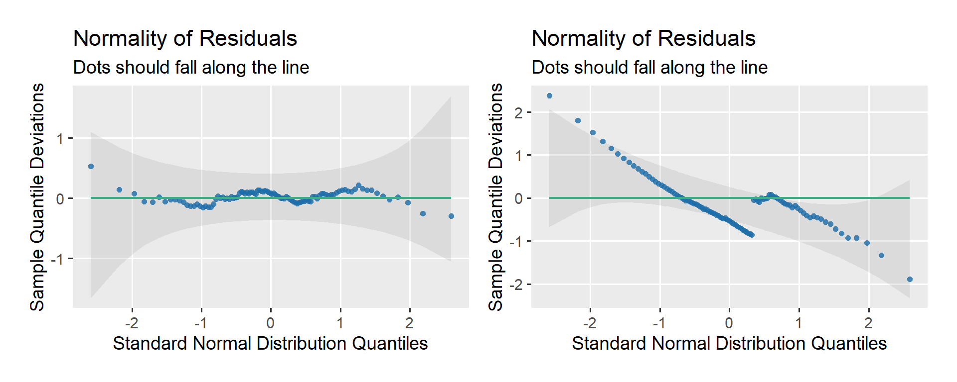
  2. Use a quantile-quantile (QQ) plot
    • Visually compare the sample and normal quantiles
    • Assumption is violated if dots stray from the line
  3. Use the Shapiro-Wilk test
    • A significant result indicates non-normality
    • But this test gets more power with a larger sample…

Example: Residual Distribution

check_model(fit_met, 
            check = "normality")
check_model(fit_violated, 
            check = "normality")
Example: QQ Plot

check_model(fit_met, 
            check = "qq")
check_model(fit_violated, 
            check = "qq")

Example: Shapiro-Wilk Test

check_normality(fit_met)
## OK: residuals appear as normally distributed (p = 0.320).

check_normality(fit_violated)
## Warning: Non-normality of residuals detected (p < .001).

Solutions

  1. Transform your outcome to be more normal
    • e.g., Box-Cox transformations
    • e.g., Yeo-Johnson transformations
  2. Use a nonparametric approach
    • e.g., nonparametric bootstrapping
    • e.g., rank-based nonparametrics
  3. Model the outcome as non-normal
    • e.g., generalized linear modeling (GLM)

Independent Residuals

Assumption

  • The residuals must be independent of (not related to) one another
    • This will be met in any random sample from a population
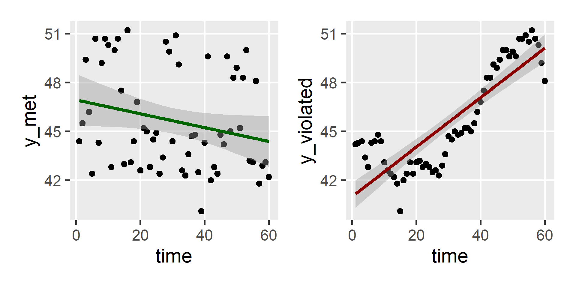
    • It will be violated with clustered or autocorrelated data
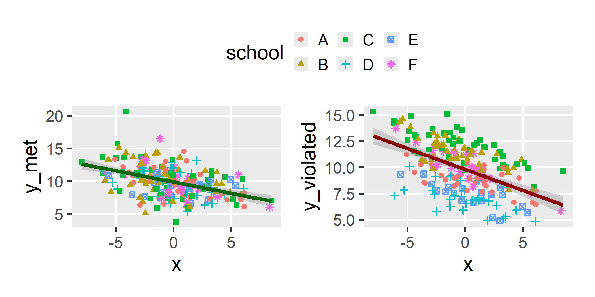
    • Clustered data has many observations from the same “group”
    • Autocorrelated data has many observations close in time

Consequences of Violating

Standard errors will be downwardly biased (i.e., deflated)

Example: Clustering

Example: Autocorrelation
Diagnostics

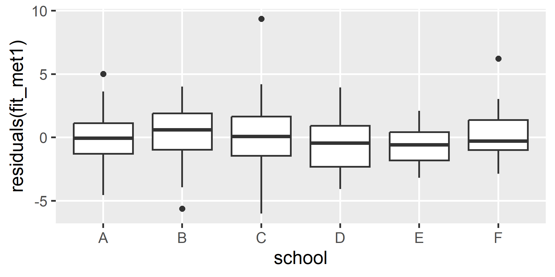
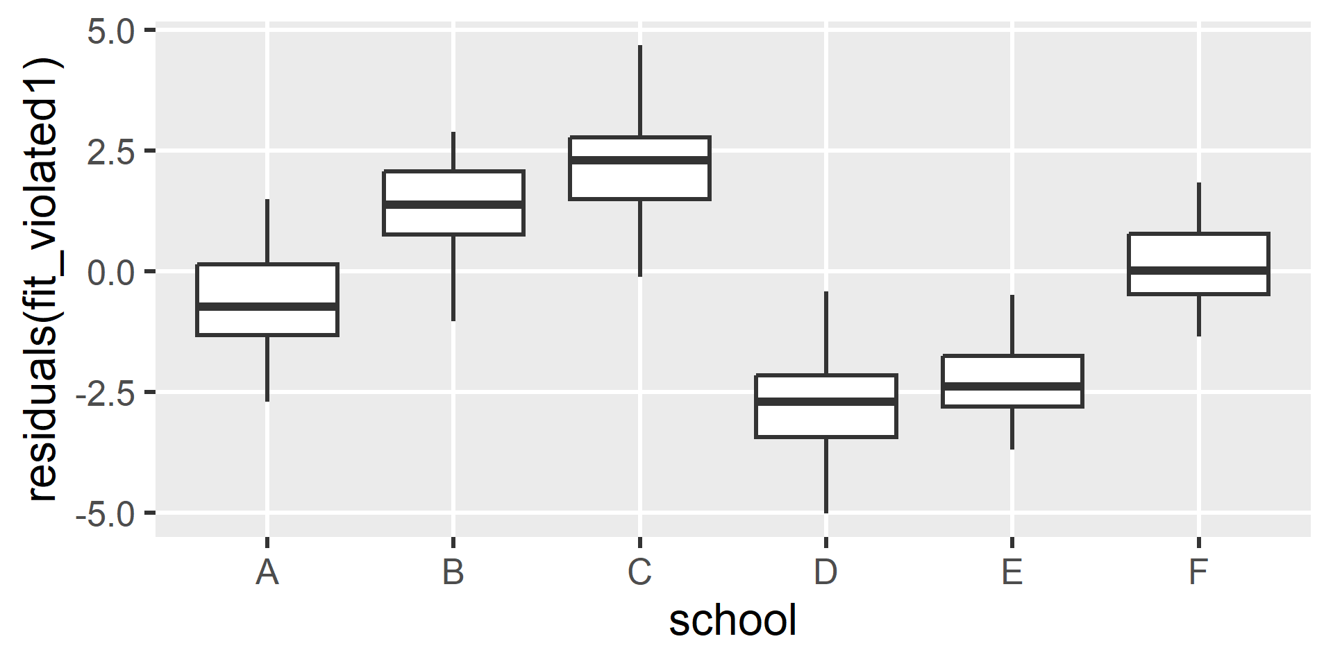
  1. If there is a potential clustering variable, do residuals differ?
    • Examine distribution of residuals in each cluster
    • Calculate a multilevel intraclass correlation
  2. Is there autocorrelation between residuals?
    • Use the Durbin-Watson serial dependency test
    • Significance indicates autocorrelation

check_autocorrelation(fit)

Example: No Clustering

qplot(x = school, y = residuals(fit_met1), data = d2a, geom = "boxplot")
Example: Clustering

qplot(x = school, y = residuals(fit_violated1), data = d2a, geom = "boxplot")
Example: Autocorrelation

check_autocorrelation(fit_met2)
## OK: Residuals appear to be independent and not autocorrelated (p = 0.416).

check_autocorrelation(fit_violated2)
## Warning: Autocorrelated residuals detected (p < .001).

Solutions

  1. Adjust the standard errors
    • e.g., cluster-robust standard errors
  2. Model the clustering explicitly
    • e.g., fixed-effects modeling
    • e.g., multilevel modeling (MLM, HLM, LME, LMM)
    • e.g., generalized estimating equations (GEE)
  3. Model the serial dependency
    • e.g., time series analysis (ARIMA)
    • e.g., autoregressive models (DSEM)

Outliers

Definition

  • Outliers are atypical observations that do not fit the other data
    • They may represent data contaminated by errors
    • Or they may represent real but rare cases
  • Outliers can have large impacts on the results of your model
    • Results may reflect the outliers rather than general patterns
  • So we need to be watchful for outliers and deal with them carefully
    • We should also be transparent about reporting our approach

Examples

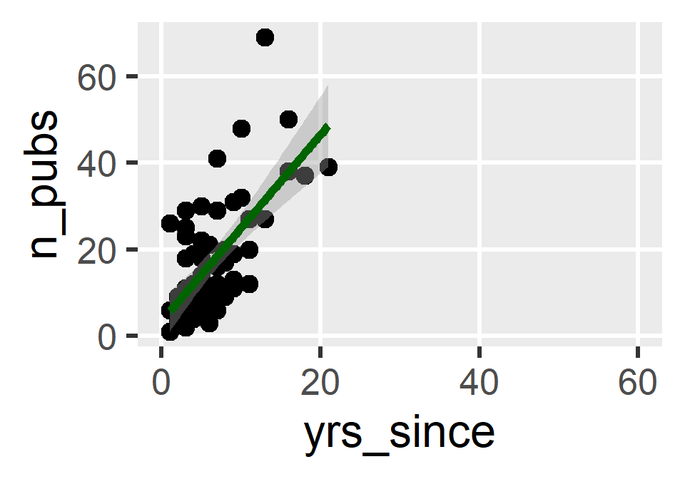
\[b_0=3.4, b_1=2.2^\ast\]

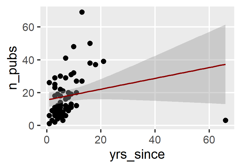
\[b_0=15.5^\ast, b_1= 0.3\]

Diagnostics

For each observation, we can calculate its…

  1. Leverage: How unusual are its \(x\) values?
    • e.g., \(h_{ii}\) and Mahalonabis distance
  2. Distance: How far is it from the regression line?
    • e.g., raw, standardized, or Studentized residuals
  3. Influence: How much does it change the coefficients?
    • e.g., \(\text{DFFITS}_i\), \(\text{DFBETAS}_i\), and Cook’s \(D_i\)

Example: No Outliers

check_outliers(fit_without, method = c("cook", "mahalanobis"))
## OK: No outliers detected.
## - Based on the following methods and thresholds: cook (0.701), mahalanobis (13.816).
## - For variable: (Whole model)

Example: With Outliers

check_outliers(fit_with, method = c("cook", "mahalanobis"))
## 1 outlier detected: case 2.
## - Based on the following methods and thresholds: cook (0.701),
##   mahalanobis (13.816).
## - For variable: (Whole model).
## 
## Note: Outliers were classified as such by at least half of the selected methods. 
## 
## -----------------------------------------------------------------------------
##  
## The following observations were considered outliers for two or more
##   variables by at least one of the selected methods:
## 
##   Row  n_Mahalanobis         n_Cook
## 1   2 (Multivariate) (Multivariate)

Solutions

  1. Fix the outliers
    • If they are errors/contaminations, fix them
  2. Keep the outliers
    • If they belong to your distribution, maybe keep them
  3. Remove the outliers
    • If they belong to a different distribution, maybe remove them
  4. Recode the outliers
    • If you want to reduce their influence, maybe Winsorize them

Remove the Outliers

If you do choose to remove the outliers, here’s how

# Number of observations before removing outliers
nrow(dat_with)
## [1] 62

# Identify outliers
outliers <- check_outliers(fit_with, method = c("cook", "mahalanobis"))

# Remove outliers
dat_drop <- dat_with[!as.numeric(outliers), ]

# Number of observations after removing outliers
nrow(dat_drop)
## [1] 61