Statistical Methods with R
Form & Collinearity
Unit D · Chapter 10 · Lecture 10a
Developed by Jeffrey M. Girard

Roadmap: Model Diagnostics
Overview
Correct Form
No Omitted Confounders
Perfect Predictors
No Collinearity
Overview
Motivation
The linear model makes certain assumptions about the data
When these assumptions are violated, two main problems occur
- Estimated coefficients (i.e., relationships) may be biased
- Intercepts and slopes directly affected
- Tests and confidence intervals indirectly affected
- Estimated standard errors (i.e., uncertainty) may be biased
- Tests and confidence intervals directly affected
- Thus, our conclusions and inferences may be incorrect!
Assumptions Overview
- Assumptions about the Formula
- Correct Functional Form
- No Omitted Confounders
- Perfectly Measured Predictors
- No Collinearity/Multicollinearity
- Assumptions about the Residuals
- Constant Error Variance
- Independence of Residuals
- Normality of Residuals
Correct Form
Assumption
- The “form” of the x-y relationship(s) must be correct
- The methods we learned so far assume straight lines
- We will also learn about polynomials for curved lines
- Advanced methods can take on other complex shapes
- This assumption is that we set up the model correctly
Consequences of Violating
Bias in both coefficients and standard errors!
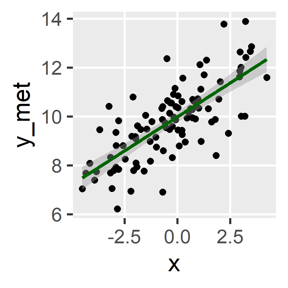
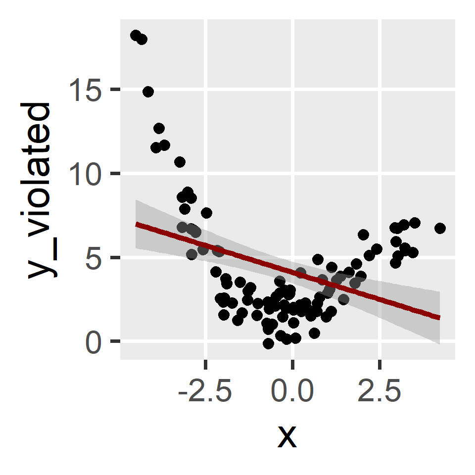
Assumption Examples
Diagnostics
- We can use scatterplots as a visual diagnostic
- A simple approach would plot y against each x
- But we can combine this into a single plot by…
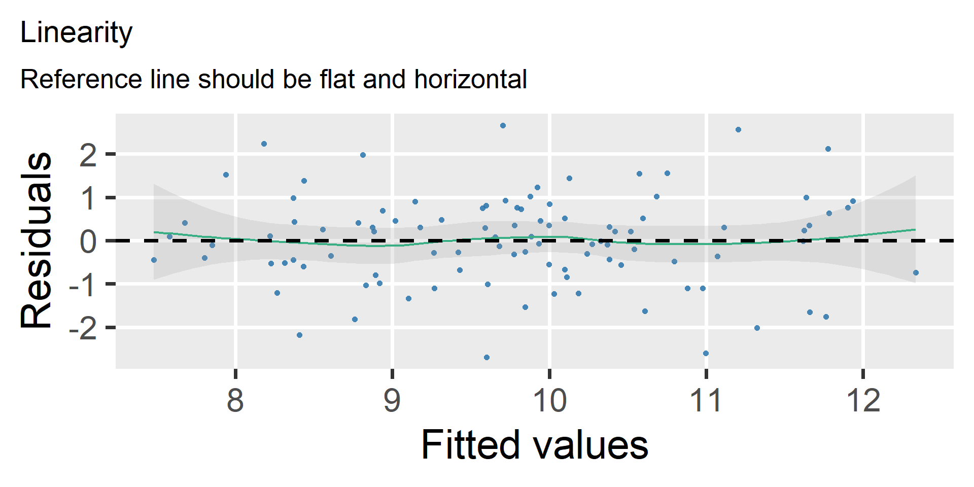
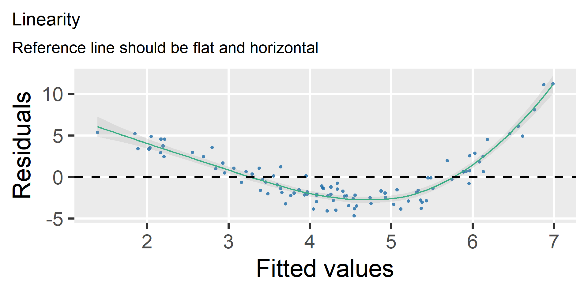
- Plot the residuals (y-\hat{y}) against the fitted values \hat{y}
- We can also add a reference (LOESS) line to these plots
- We want to see a flat and horizontal reference line
check_model(fit, check = "linearity")
With several predictors, a curve in one x can be diluted here; per-predictor residual plots help
Example: Assumption Met
Example: Assumption Violated
Solutions
- Specify a more complex functional form
- e.g., variable transformations
- e.g., polynomial regression
- e.g., segmented or piece-wise regression
- Use a nonlinear extension of regression
- e.g., generalized linear modeling (GLM)
- e.g., generalized additive modeling (GAM)
- e.g., supervised machine learning (ML)
No Omitted Confounders
Assumption
- Any cause of y that correlates with an x must be in the model
- Such a variable is called a confounder
- Its effect does not vanish; the predictors you kept absorb it
- We saw this in Chapter 07c: leaving
educationout made White Collar look more prestigious than Blue Collar, and putting it back reversed the sign
Consequences of Violating
Bias in the coefficients, and therefore in the tests and intervals built on them!
Diagnostics
- There is no diagnostic plot for this one
- A confounded model can have perfect-looking residuals
- Nothing in the data can reveal a variable that is not in the data
- Instead, we argue from theory and design
- What else plausibly causes y?
- Is it correlated with any predictor we care about?
- Did we measure it?
This is the assumption you cannot test, only defend.
Solutions
- Measure and include the confounder
- Decided at design time, not analysis time
- Remove the confounding by design
- e.g., random assignment to conditions
- e.g., matching or restriction
- Be honest about what is left
- Report plausible confounders you could not measure
- Describe effects as adjusted for what you included, not as causal
Do not “control for everything”: adjusting for a mediator removes the very pathway you are studying.
Perfect Predictors
Assumption
- All predictors (x) must be measured without error
- With a single predictor, the slope will be underestimated
- With many predictors, slopes may be too low or high
- When violated, called regression “dilution” or “attenuation”
Consequences of Violating
Bias in both coefficients and standard errors!
Error in y will bias standardized (but not unstandardized) coefficients.
Diagnostics
Calculate predictors’ reliability (the opposite of error)
- Test-retest reliability across time
- Correlation from
correlation::correlation()
- Correlation from
- Internal reliability across items
- McDonald’s Omega from
psych::omega()
- McDonald’s Omega from
- Inter-rater reliability across raters
- Intraclass Correlation from
irr::icc()
- Intraclass Correlation from
Solutions
- Improve measurement reliability
- e.g., add items, raters, or training
- Adjust coefficients for reliability
- e.g., correlation disattenuation
- Model reliability/error explicitly
- e.g., total least squares estimation
- e.g., errors-in-variables models
- e.g., structural equation modeling
No Collinearity
Assumption
- No set of predictors are redundant with one another
- Collinearity = 2 predictors, Multicollinearity = 3+
- If x_1 and x_2 fully overlap, there are no partial effects left
- The model won’t fit (or drops one or more predictors)
- If they almost fully overlap, the estimates become unstable
Consequences of Violating
Coefficients stay unbiased but become unstable; standard errors become larger, honestly reflecting that instability.
Unstable means the estimate swings a lot from sample to sample, not that it is systematically too high or too low.
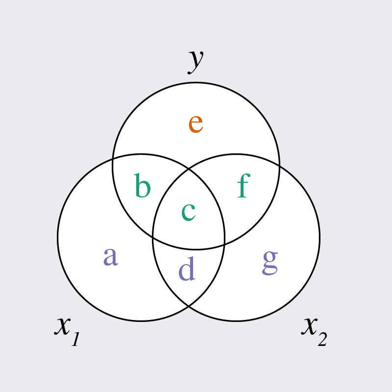
Assumption
If x_1 and x_2 overlap to a
very large degree, then…
- c and/or d are large
- b and f are unstable
\hat{y} = b_0 + b_1x_1 + b_2x_2
- So b_1 and b_2 are unstable
Diagnostics
- Examine predictor correlations for collinearity
- r(x_1, x_2)\ge0.9 may be problematic
- But no cutoff maps cleanly onto SE inflation
- It also doesn’t detect multicollinearity
- Calculate variance inflation factors (VIFs)
- Look for evidence of inflated standard errors
- Each predictor will get its own VIF value
- \text{VIF}>5 is “moderate”, \text{VIF}>10 is “high”
Variance Inflation Factors
- To calculate the \text{VIF} for predictor j…
- Regress x_j on all other predictors
- Calculate R^2 from that model
- Calculate \text{VIF} from that R^2
\text{VIF}_j = \frac{1}{1-R^2_j}
check_collinearity(fit)
Example Data
Let’s simulate data with collinearity problems
Simulated Data
y(Continuous)height1,height2,weight,size(Continuous)female,male(Binary)
Simulated Issues
height2mirrorsheight1sizeis multicollinear withheight1andweightmaleduplicatesfemale
Bivariate Correlations
round(cor(simdat), digits = 2)
##         height1 height2 weight  size female  male     y
## height1    1.00    0.97   0.07  0.72   0.15 -0.15  0.33
## height2    0.97    1.00   0.09  0.71   0.14 -0.14  0.29
## weight     0.07    0.09   1.00  0.72   0.16 -0.16 -0.66
## size       0.72    0.71   0.72  1.00   0.23 -0.23 -0.22
## female     0.15    0.14   0.16  0.23   1.00 -1.00 -0.05
## male      -0.15   -0.14  -0.16 -0.23  -1.00  1.00  0.05
## y 0.33 0.29 -0.66 -0.22 -0.05 0.05 1.00height1andheight2are highly correlated (r=.97)femaleandmaleare perfectly correlated (r=-1.00)However,
sizeis not as correlated withheight1(r=.72)
orweight(r=.72) despite the three being multicollinear
Example with No Issues
fit_none <- lm(y ~ height1 + weight, data = simdat)

model_parameters(fit_none)
## Parameter   | Coefficient |   SE |         95% CI |  t(97) |      p
## -------------------------------------------------------------------
## (Intercept) |       10.02 | 0.12 | [ 9.80, 10.25] |  87.06 | < .001
## height1     |        0.20 | 0.04 | [ 0.13,  0.28] |   5.53 | < .001
## weight      |       -0.38 | 0.04 | [-0.45, -0.30] | -10.16 | < .001

r2(fit_none)
## # R2 for Linear Regression
##        R2: 0.567
## adj. R2: 0.558- Both slopes are significant
- The SE of both slopes is 0.04
- The R^2 is 0.567 (57%)
Example with No Issues
Let’s calculate the VIFs for this model
- The VIFs for both predictors are low (<5)
Example with Collinearity
fit_co <- lm(y ~ height1 + weight + height2, data = simdat)

model_parameters(fit_co)
## Parameter   | Coefficient |   SE |         95% CI |  t(96) |      p
## -------------------------------------------------------------------
## (Intercept) |       10.02 | 0.12 | [ 9.79, 10.25] |  86.61 | < .001
## height1     |        0.24 | 0.15 | [-0.05,  0.53] |   1.61 | 0.110
## weight      |       -0.38 | 0.04 | [-0.45, -0.30] | -10.04 | < .001
## height2     |       -0.03 | 0.15 | [-0.32,  0.26] |  -0.23 | 0.821

r2(fit_co)
## # R2 for Linear Regression
##        R2: 0.567
## adj. R2: 0.553- The
height1slope is no longer significant - The SE of the height slopes are both 0.15 (up from 0.04)
- Note that the R^2 is basically the same (57%)
Example with Collinearity
Let’s calculate the VIFs for this model
check_collinearity(fit_co)
## # Check for Multicollinearity
##
## Low Correlation
##
##    Term  VIF       VIF 95% CI adj. VIF Tolerance Tolerance 95% CI
##  weight 1.01 [ 1.00, 5128.00]     1.01      0.99     [0.00, 1.00]
##
## High Correlation
##
##     Term   VIF       VIF 95% CI adj. VIF Tolerance Tolerance 95% CI
##  height1 15.71 [11.06,   22.49]     3.96      0.06     [0.04, 0.09]
## height2 15.76 [11.10, 22.58] 3.97 0.06 [0.04, 0.09]- The VIFS for both height variables are very high (>10)
Example with Multicollinearity
fit_mc <- lm(y ~ height1 + weight + size, data = simdat)

model_parameters(fit_mc)
## Parameter   | Coefficient |   SE |         95% CI | t(96) |      p
## ------------------------------------------------------------------
## (Intercept) |       10.02 | 0.12 | [ 9.79, 10.25] | 85.93 | < .001
## height1     |        0.24 | 0.18 | [-0.11,  0.60] |  1.37 | 0.175
## weight      |       -0.34 | 0.18 | [-0.69,  0.01] | -1.92 | 0.058
## size        |       -0.04 | 0.18 | [-0.39,  0.31] | -0.22 | 0.828

r2(fit_mc)
## # R2 for Linear Regression
##        R2: 0.567
## adj. R2: 0.553- None of the slopes are significant
- The SE of all slopes is now 0.18 (up from 0.04)
- Note that the R^2 is basically the same (57%)
Example with Multicollinearity
Let’s calculate the VIFs for this model
check_collinearity(fit_mc)
## # Check for Multicollinearity
##
## High Correlation
##
##     Term   VIF     VIF 95% CI adj. VIF Tolerance Tolerance 95% CI
##  height1 22.91 [16.05, 32.89]     4.79      0.04     [0.03, 0.06]
##   weight 22.60 [15.84, 32.44]     4.75      0.04     [0.03, 0.06]
## size 47.41 [33.03, 68.25] 6.89 0.02 [0.01, 0.03]- The VIFs for all predictors are very high (>10)
Example with Exact Collinearity
fit_xc <- lm(y ~ female + male, data = simdat)

model_parameters(fit_xc)
## Model matrix is rank deficient. Parameters `male` were not estimable.
## Parameter   | Coefficient |   SE |         95% CI | t(98) |      p
## ------------------------------------------------------------------
## (Intercept) |       10.01 | 0.24 | [ 9.52, 10.49] | 40.89 | < .001
## female      |       -0.19 | 0.34 | [-0.87,  0.49] | -0.54 | 0.590
##
## Uncertainty intervals (equal-tailed) and p-values (two-tailed) computed
## using a Wald t-distribution approximation.- Note the warning about the
maleparameter - Note the absence of a
maleslope (it was dropped) - This is why we use (g-1) dummy codes and not g
Solutions
- Break the predictors’ redundancy
- e.g., drop one or more predictors
- e.g., combine two or more predictors
- e.g., reduce predictor dimensionality (PCA)
- e.g., penalized (lasso or ridge) regression
- Model the predictors’ shared variance
- e.g., partial least squares estimation
- e.g., structural equation modeling