Statistical Methods with R

Polynomial Regression

Unit C · Chapter 09 · Lecture 09a

Developed by Jeffrey M. Girard

Overview

Motivation

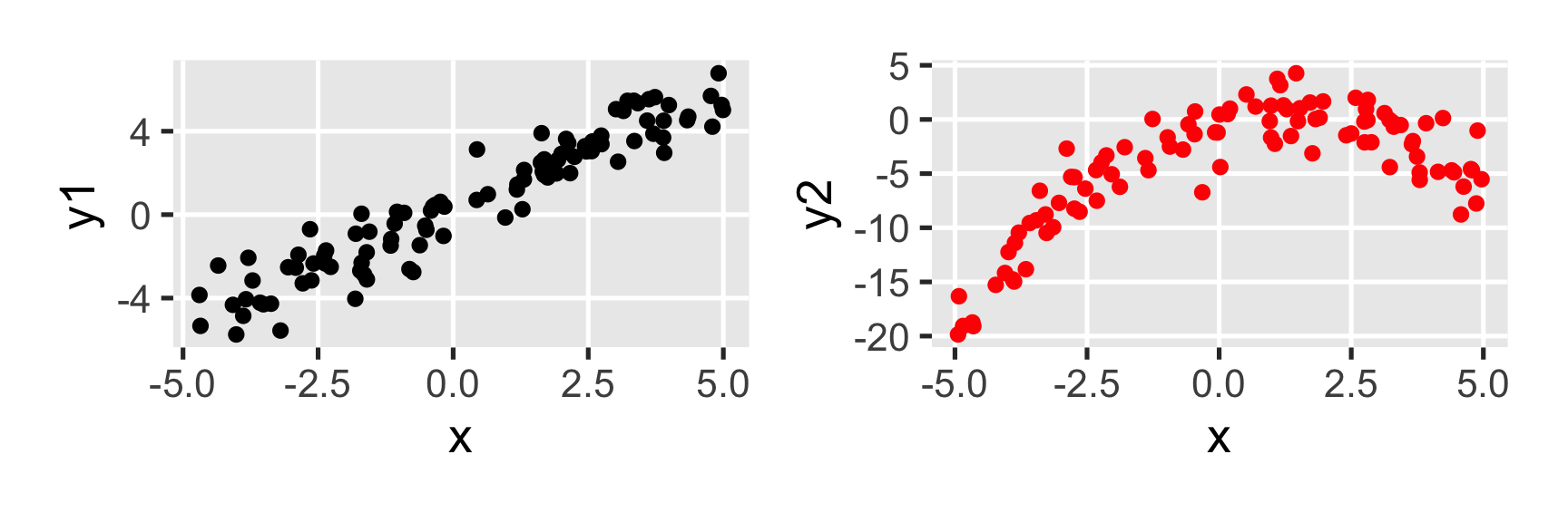
• So far, we have always fit straight lines between \(y\) and \(x\) variables

• But sometimes the correct functional form is curved in some way

• If we fit a straight line anyway, our results may be very biased

Linear regression

fit <- lm(y2 ~ x, data = df2) # data from right panel of slide 3

model_parameters(fit)
## Parameter   | Coefficient |   SE |         95% CI |  t(98) |      p
## -------------------------------------------------------------------
## (Intercept) |       -4.54 | 0.43 | [-5.39, -3.70] | -10.66 | < .001
## x           |        1.19 | 0.14 | [ 0.90,  1.47] |   8.29 | < .001

r2(fit)
## # R2 for Linear Regression
##        R2: 0.412
##   adj. R2: 0.406

Visualizing the model

library(modelbased)
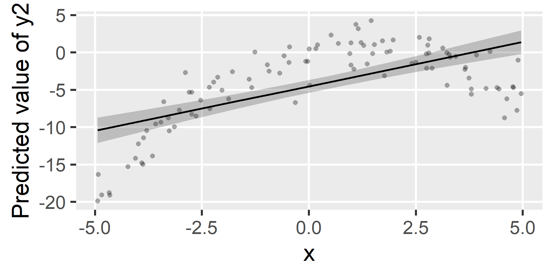
plot(estimate_relation(fit, by = "x"), show_data = TRUE)

Assumption checking

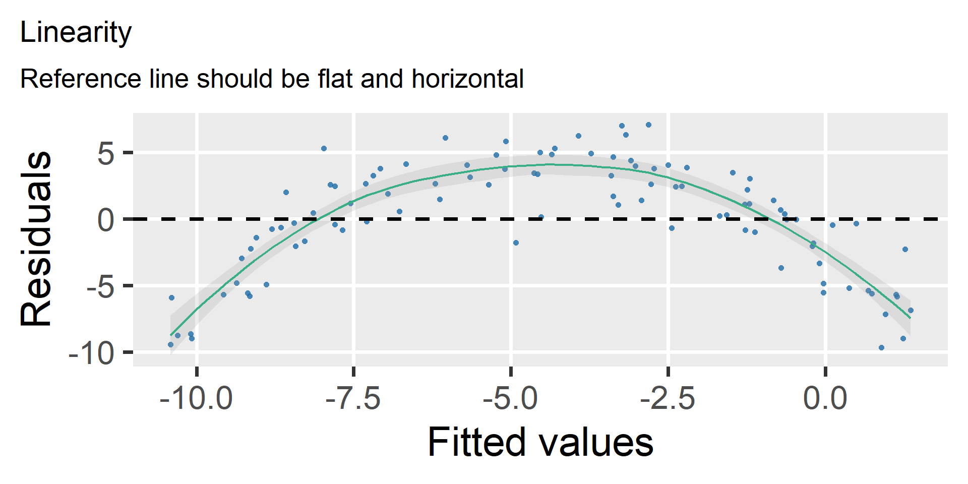
check_model(fit, check = "linearity")

Conclusions

• Linear regression did not work well for predicting \(y_2\)

• The functional form diagnostic looked bad for the latter

• The \(R^2\) for the latter was worse than we could do

• We need to change our functional form!

• We need to allow a curve in our function

• This is what polynomial regression does

Polynomial Regression

Power polynomials

• LM can handle simple curves through power polynomial transformations!

• We will add predictors that are power transformations of other predictors

\[\hat{y} = b_0 + b_1 \color{red}{x^1} + b_2 \color{red}{x^2} + \cdots + b_d \color{red}{x^d}\]

• Each term has a degree equal to its exponent
  • e.g., \(x^1\) is the first degree term and \(x^2\) is the second degree term
  • Note that \(x^1=x\) and \(x^0=1\), which can be thought of as the intercept
  • The term with the highest exponent is the highest degree term
  • All other terms are referred to as the lower degree terms

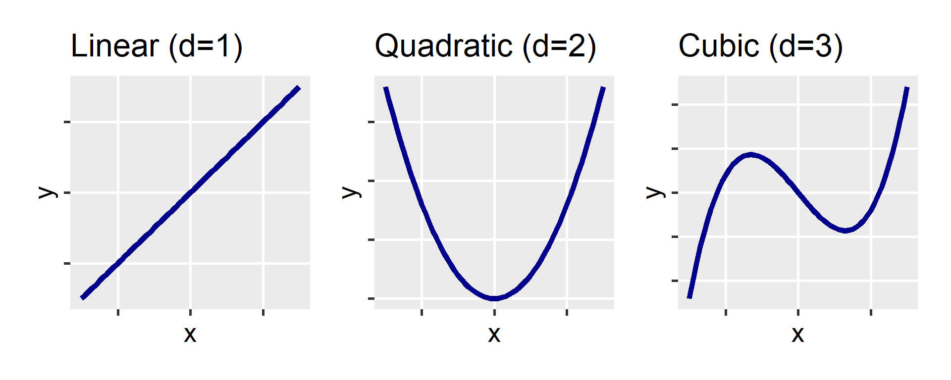
Number of bends

• The highest degree term determines the curve’s overall shape
  • The number of bends is equal to \((d-1)\)

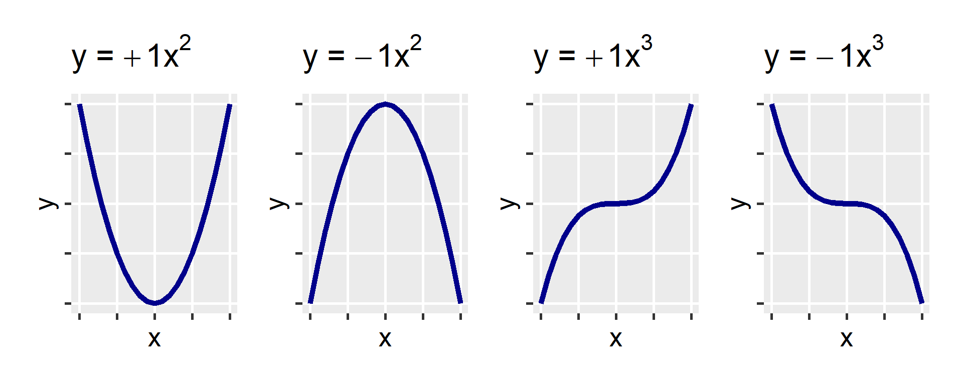
Direction of curvature

• The sign \((\pm)\) of the curve’s highest degree term’s slope
  determines its direction of curvature (i.e., up or down)

Quadratic Regression

Expanding the equation

• A quadratic relationship requires two predictors to represent \(x\)

\[\hat{y} = b_0 + b_1 x^1 + b_2 x^2\]

• The highest degree coefficient determines the overall shape
  • \(b_2\): Does the curve bend up \((+)\), down \((-)\), or not at all \((0)\)?

• The lower degree coefficients fine-tune the position and shape
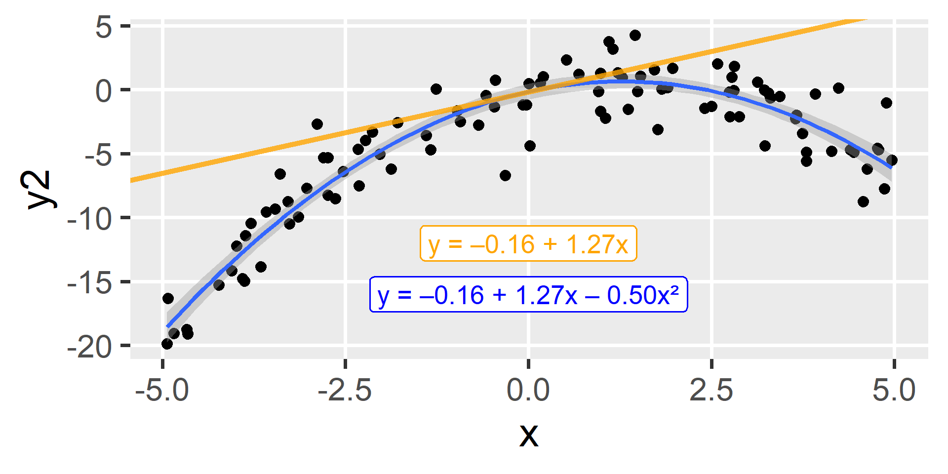
  • \(b_1\): What is the slope of the curve’s tangent line at \(x=0\)?
  • \(b_0\): What is the intercept of the curve’s tangent line at \(x=0\)?

Quadratic regression 1

• We use the I() function to do math inside the formula

fit1b <- lm(y1 ~ x + I(x^2), data = df1)

model_parameters(fit1b)
## Parameter   | Coefficient |   SE |        95% CI | t(97) |      p
## -----------------------------------------------------------------
## (Intercept) |        0.27 | 0.15 | [-0.02, 0.57] |  1.82 | 0.072 
## x           |        1.13 | 0.04 | [ 1.05, 1.20] | 30.43 | < .001
## x^2         |    3.05e-03 | 0.01 | [-0.03, 0.03] |  0.21 | 0.838

r2(fit1b)
## # R2 for Linear Regression
##        R2: 0.908
##   adj. R2: 0.906

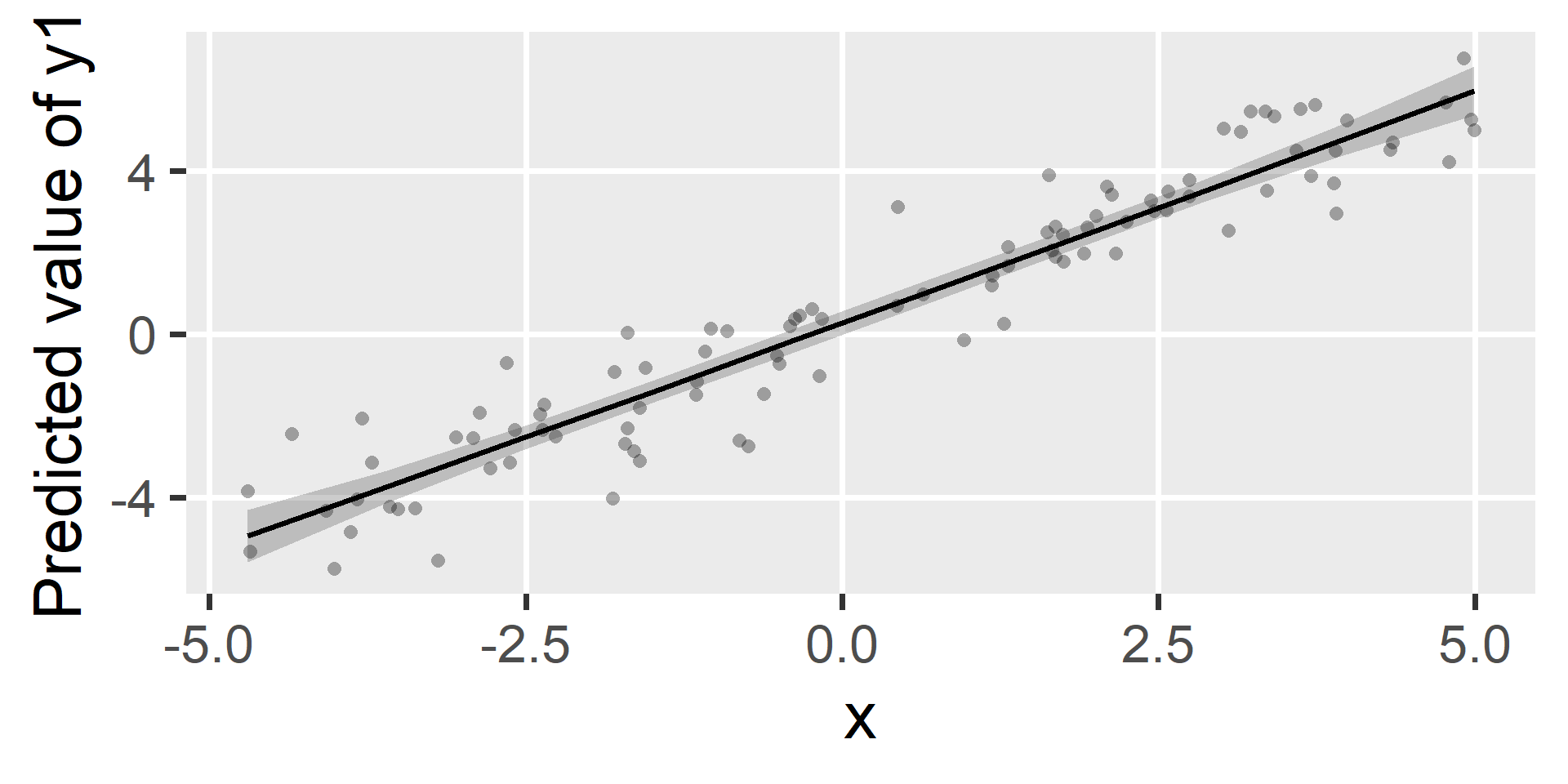
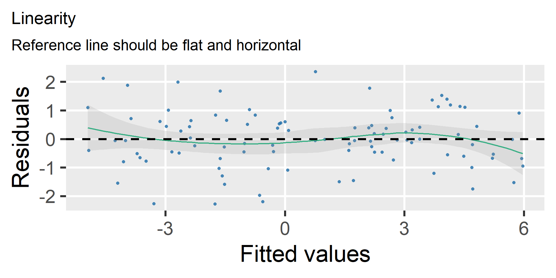
The \(x^2\) slope is NOT significant, so the curve is NOT needed

Visualizing the model

plot(estimate_relation(fit1b, by = "x"), show_data = TRUE)

Assumption checking

check_model(fit1b, check = "linearity")

Quadratic regression 2

fit2b <- lm(y2 ~ x + I(x^2), data = df2)

model_parameters(fit2b)
## Parameter   | Coefficient |   SE |         95% CI |  t(97) |      p
## -------------------------------------------------------------------
## (Intercept) |       -0.16 | 0.31 | [-0.77,  0.45] |  -0.53 | 0.599 
## x           |        1.27 | 0.07 | [ 1.13,  1.40] |  18.85 | < .001
## x^2         |       -0.50 | 0.03 | [-0.55, -0.44] | -18.71 | < .001

r2(fit2b)
## # R2 for Linear Regression
##        R2: 0.872
##   adj. R2: 0.870

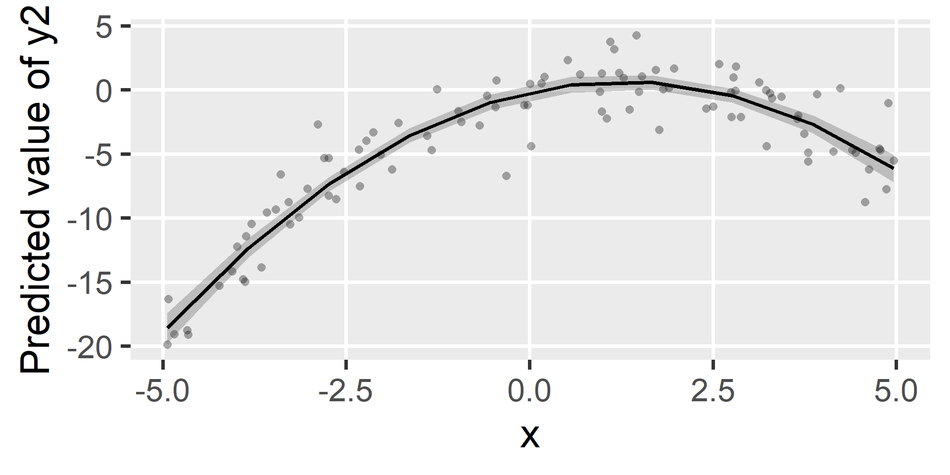
• The \(x^2\) slope is significant, so the curve is needed!
• Because the slope is negative, it will bend downward

Visualizing the model

plot(estimate_relation(fit2b, by = "x"), show_data = TRUE)

Assumption checking

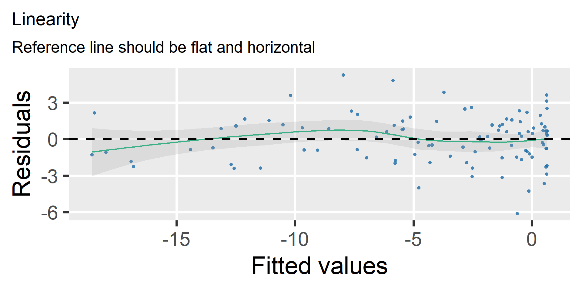
check_model(fit2b, check = "linearity")

Visualizing the tangent line

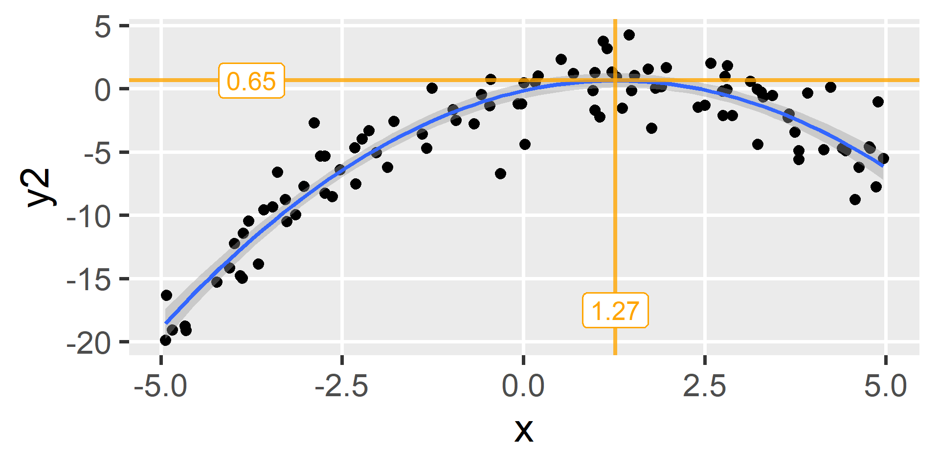
Calculating extrema

• It may be useful to know the maximum or minimum values

What value of \(x\) gives the
most extreme value of \(y\)?

\[x_m = \frac{-b_1}{2b_2}\]

What is the most extreme value of \(y\) in the function?

\[\hat{y}_m = \frac{4 b_2 b_0 - b_1^2}{4 b_2}\]

Calculating extrema

model_parameters(fit2b)
## Parameter   | Coefficient |   SE |         95% CI |  t(97) |      p
## -------------------------------------------------------------------
## (Intercept) |       -0.16 | 0.31 | [-0.77,  0.45] |  -0.53 | 0.599 
## x           |        1.27 | 0.07 | [ 1.13,  1.40] |  18.85 | < .001
## x^2         |       -0.50 | 0.03 | [-0.55, -0.44] | -18.71 | < .001

b_0 <- -0.16
b_1 <-  1.27
b_2 <- -0.50

x_m <- (-b_1) / (2 * b_2)
x_m
## [1] 1.27

yhat_m <- ((4 * b_2 * b_0) - b_1^2) / (4 * b_2)
yhat_m
## [1] 0.64645

Visualizing extrema

Adding Predictors

Adding another predictor

library(tidyverse)
penguins <- read_csv("../../data/penguins.csv")

fit3 <- lm(
  body_mass ~ flipper_len + I(flipper_len^2) + sex,
  data = penguins
)

model_parameters(fit3)
## Parameter     | Coefficient |      SE |              95% CI | t(329) |      p
## -----------------------------------------------------------------------------
## (Intercept)   |    15151.13 | 4175.96 | [6936.18, 23366.08] |   3.63 | < .001
## flipper len   |     -156.15 |   41.19 | [-237.18,   -75.12] |  -3.79 | < .001
## flipper len^2 |        0.50 |    0.10 | [   0.30,     0.70] |   4.93 | < .001
## sex [male]    |      337.83 |   39.04 | [ 261.03,   414.62] |   8.65 | < .001

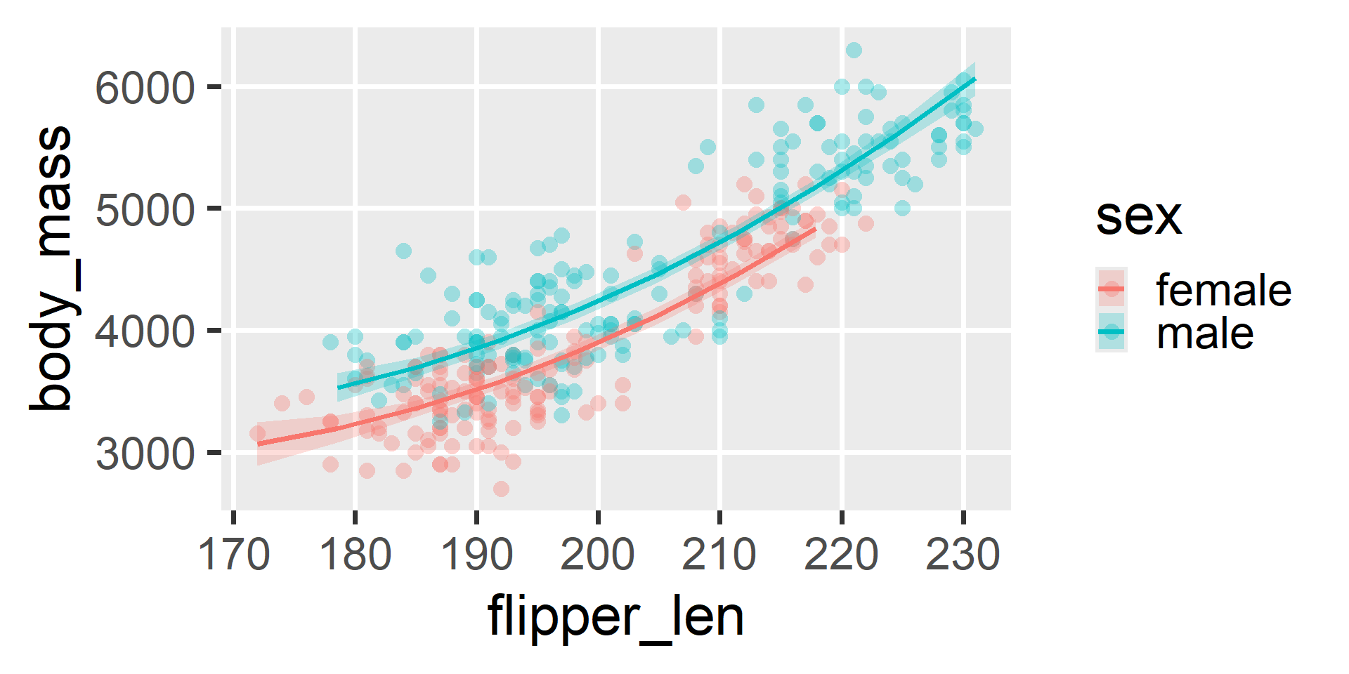
• The effects of flipper_len are significant controlling for sex

• The effect of sex is significant controlling for flipper_len and its square

Visualizing the model

plot(estimate_relation(fit3, by = c("flipper_len", "sex")), show_data = TRUE)

Adding moderation

fit4 <- lm(
  body_mass ~ flipper_len + I(flipper_len^2) + sex +
    flipper_len:sex + I(flipper_len^2):sex,
  data = penguins
)

model_parameters(fit4)
## Parameter                  | Coefficient |       SE |                95% CI
## ---------------------------------------------------------------------------
## (Intercept)                |    32222.60 |  7935.58 | [ 16611.37, 47833.84]
## flipper len                |     -332.67 |    79.94 | [  -489.93,  -175.41]
## flipper len^2              |        0.95 |     0.20 | [     0.56,     1.35]
## sex [male]                 |   -13238.21 | 10025.40 | [-32960.64,  6484.21]
## flipper len × sex [male]   |      145.66 |    99.69 | [   -50.45,   341.78]
## flipper len^2 × sex [male] |       -0.39 |     0.25 | [    -0.87,     0.10]
## 
## Parameter                  | t(327) |      p
## --------------------------------------------
## (Intercept)                |   4.06 | < .001
## flipper len                |  -4.16 | < .001
## flipper len^2              |   4.75 | < .001
## sex [male]                 |  -1.32 | 0.188 
## flipper len × sex [male]   |   1.46 | 0.145 
## flipper len^2 × sex [male] |  -1.57 | 0.118

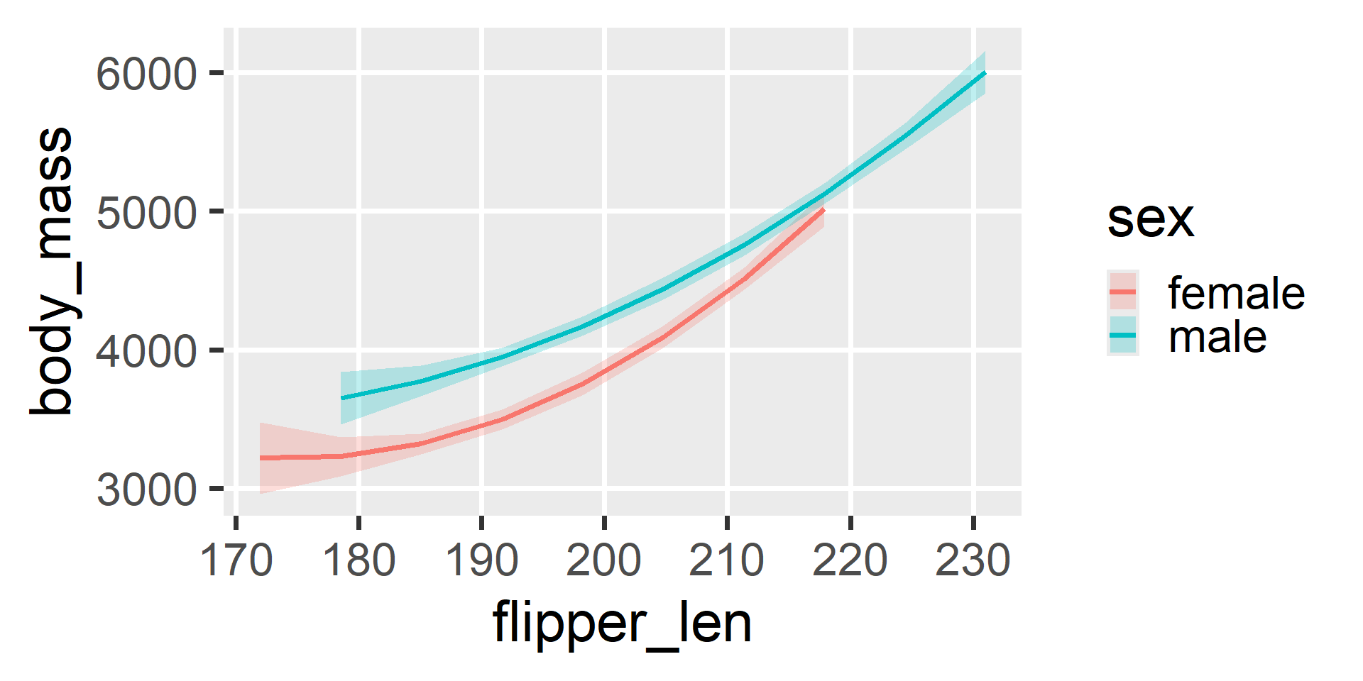
• The effects of flipper_len are not moderated by sex

Visualizing the model

plot(estimate_relation(fit4, by = c("flipper_len", "sex")))

Closing Thoughts

Consider the range

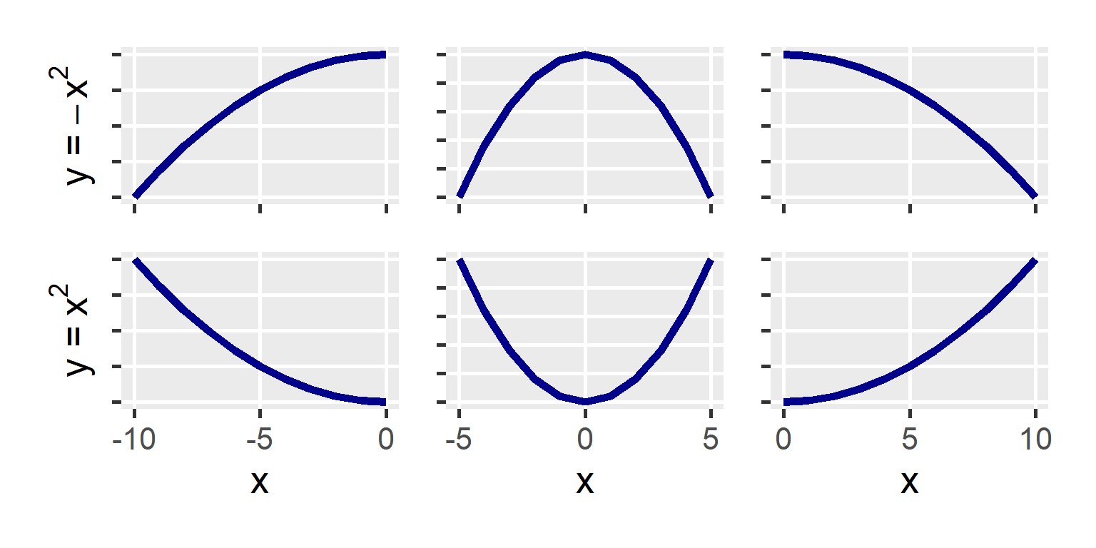
• You may only see part of the curve in your sample!

Advice

• Models with higher degrees are more flexible
  • But they may overfit (fail to generalize)
  • They will be harder to interpret and justify
• Theory should be used to decide between shapes
  • Quadratics can model processes with best/worst regions
  • Cubics can model opponent processes and regulation
• Centering your \(x\) variable is very helpful here
  • Also see poly() for orthogonal polynomials
• Don’t omit the lower degree terms/coefficients