library(tidyverse)
exercise <- read_csv("exercise.csv")

fit <- lm(expenditure ~ duration * sex, data = exercise)
model_parameters(fit)
## Parameter             | Coefficient |   SE |         95% CI | t(896) |     p
## ----------------------------------------------------------------------------
## (Intercept)           |        3.33 | 2.73 | [-2.02,  8.69] |   1.22 | 0.222
## duration              |        3.32 | 1.33 | [ 0.70,  5.93] |   2.49 | 0.013
## sex [male]            |        3.57 | 3.91 | [-4.11, 11.25] |   0.91 | 0.362
## duration × sex [male] | -1.72 | 1.90 | [-5.45, 2.00] | -0.91 | 0.364Statistical Methods with R
Categorical Moderation
Unit C · Chapter 08 · Lecture 08b
Developed by Jeffrey M. Girard
Roadmap: Moderation
Review
Binary-by-Continuous
Nominal-by-Continuous
Categorical-by-Categorical
Three-Way Interactions
Review
Review of Last Lecture
We learned about moderation via interaction terms
The interaction effect is the slope of the product x_1 x_2
- This allows the slope of x_1 to depend on the value of x_2
- (and vice versa, slope of x_2 on value of x_1)
We focused on interactions between continuous variables
- There were infinite slopes (one for each value of x_2)
- So we chose to “spotlight” just a few possible slopes
Example moderation questions
Continuous-by-Continuous Interaction
- Does the effect of
durationonexpendituredepend onintensity?
Continuous-by-Categorical Interaction
- Does the effect of
durationonexpendituredepend onsex?
Categorical-by-Categorical Interaction
- Does the effect of
programonexpendituredepend onsex?
Higher-Order Interaction
- Does the interaction of
durationandintensitydepend onsex?
Binary-by-Continuous
Motivation
- Can we interact categorical and continuous predictors?
- Yes! In fact, in some ways, it is even easier than before
- Instead of infinite slopes, we have one slope per category
- Let’s moderate a continuous predictor by a binary variable
- Does the effect of
durationdiffer bysex? - Perhaps exercise is more “costly” for men or women…
- Does the effect of
Adding Interaction Term
- If x_1 is continuous and x_2 is binary, we can dummy code x_2
- c_1=0 for the reference group (x_2= female)
- c_1=1 for the non-reference group (x_2= male)
- We then add an interaction term x_1 c_1 with its own slope
\hat{y} = b_0 + b_1 x_1 + b_2 c_1 + b_3 x_1 c_1
formula = expenditure ~ duration * sex
Interpreting the Coefficients
\hat{y} = b_0 + b_1 x_1 + b_2 c_1 + b_3 x_1 c_1
b_0 (intercept): the predicted value of y when x_1=0 and c_1=0
b_1 (simple): the change in y expected for a change of +1 in x_1 (at c_1=0)
b_2 (simple): the difference in y between the two x_2 groups (at x_1=0)
b_3 (interaction): two equivalent definitions
- the difference in b_1 (i.e., the slope of x_1) between the two x_2 groups
- the difference in b_2 (i.e., the difference between the two x_2 groups) expected for a change of +1 in x_1
Rearranging the Formula
\hat{y} = b_0 + b_1 x_1 + b_2 c_1 + b_3 x_1 c_1
\hat{y} = b_0 + (b_1 + b_3 c_1) x_1 + b_2 c_1
Thus, the slope of x_1 (its multiplier) depends on the x_2 group
Also, if there is no interaction (b_3=0), then b_1 is unchanged
The same is true for the slope of c_1 if we rearrange again
\hat{y} = b_0 + b_1 x_1 + (b_2 + b_3 x_1) c_1
Interaction and Simple Effects
The interaction effect (duration \times sex) is NOT significant
Thus, we have no evidence that the effect of
durationdepends onsex
Predicting energy expenditure
\hat{y} = 3.33 + 3.32 x_1 + 3.57 c_1 - 1.72 x_1 c_1
Intercept: A female participant exercising at 0 duration expends 3.33 units
Duration Simple Effect: Each unit of duration expends 3.32 units more (for females)
Sex Simple Effect: Males will expend 3.57 units more than females (at 0 duration)
Interaction Effect: The slope of duration will decrease by 1.72 for males, and the male–female difference will decrease by 1.72 for each added unit of duration
The average participant (2 duration) expends 9.97 units (female) or 10.1 units (male)
\text{Female: }\hat{y} = 3.33 + 3.32(2) + 3.57(0) - 1.72(2)(0) = 9.97 \text{Male: }\hat{y} = 3.33 + 3.32(2) + 3.57(1) - 1.72(2)(1) = 10.10
Plotting interaction effects
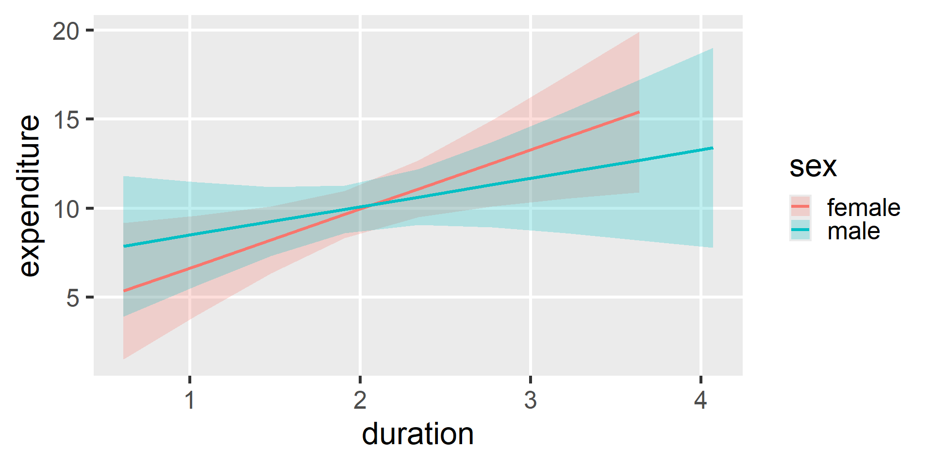
You can tell there is not a significant interaction because the lines could be parallel.
Plotting interaction effects
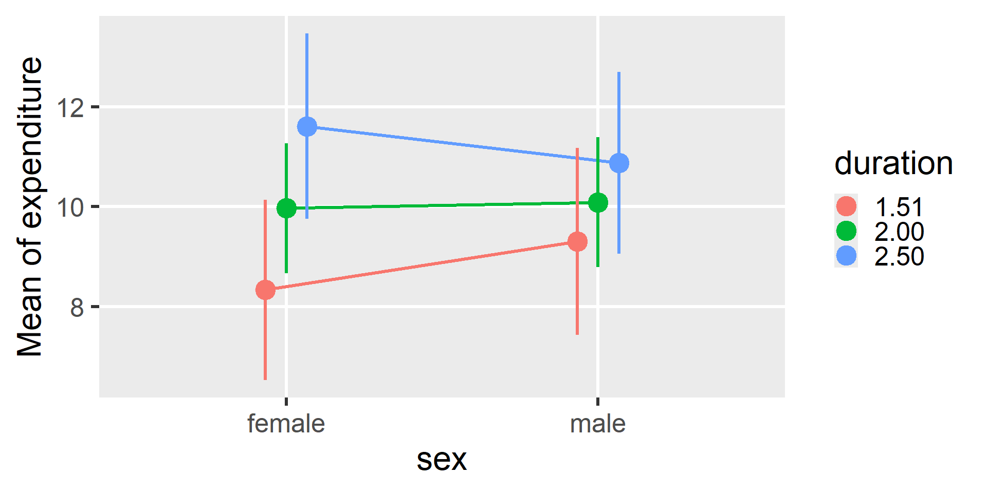
You can still spotlight duration but then you lose some information.
Simple slopes
- What is the slope of
durationin eachsexgroup?
estimate_slopes(fit, trend = "duration", by = "sex")
## Estimated Marginal Effects
##
## sex    | Slope |   SE |        95% CI | t(896) |     p
## ------------------------------------------------------
## female |  3.32 | 1.33 | [ 0.70, 5.93] |   2.49 | 0.013
## male   |  1.59 | 1.35 | [-1.06, 4.25] |   1.18 | 0.240
##
## Marginal effects estimated for duration
## Type of slope was dY/dX
Marginal Contrasts
- Is the
sexdifference significant at any value ofduration?- Usually only do this if the interaction is significant
estimate_contrasts(fit, contrast = "sex", by = "duration = [sd]")
## Marginal Contrasts Analysis
##
## Level1 | Level2 | duration | Difference |   SE |        95% CI | t(896) |     p
## -------------------------------------------------------------------------------
## male   | female |     1.51 |       0.97 | 1.33 | [-1.63, 3.58] |   0.73 | 0.464
## male   | female |     2.00 |       0.12 | 0.94 | [-1.72, 1.96] |   0.13 | 0.898
## male   | female |     2.50 |      -0.73 | 1.33 | [-3.34, 1.87] |  -0.55 | 0.580
##
## Variable predicted: expenditure
## Predictors contrasted: sex
## p-values are uncorrected.
Reporting Results
We used a linear model to regress the continuous energy expenditure variable on the continuous exercise duration variable, the binary biological sex variable (dummy coded as 0=female, 1=male), and the duration-by-sex interaction.
The simple slope of duration was significant for females (p=.013) but not for males (p=.240) and the simple slope of sex was not significant at 0 duration (p=.362). The duration-by-sex interaction was not significant (p=.364).
Dropping the interaction
- Unless the interaction was my main research question, I might drop a non-significant interaction and re-estimate the model to get partial effects (rather than simple effects)
fit2 <- lm(expenditure ~ duration + sex, data = exercise)
model_parameters(fit2)
## Parameter   | Coefficient |   SE |        95% CI | t(897) |     p
## -----------------------------------------------------------------
## (Intercept) |        5.02 | 2.00 | [ 1.10, 8.95] |   2.51 | 0.012
## duration    |        2.47 | 0.95 | [ 0.60, 4.33] |   2.60 | 0.009
## sex [male]  |        0.12 | 0.94 | [-1.72, 1.96] |   0.13 | 0.899
Nominal-by-Continuous
Expanding the equation
- The same approach applies for a nominal moderator
- But needs multiple dummy codes and interaction terms
\hat{y} = b_0 + b_1 x_1 + b_2 c_1 + b_3 c_2 + b_4 x_1 c_1 + b_5 x_1 c_2
formula = expenditure ~ duration * program
(program \in\{\text{jog, swim, read}\} needs 2 dummy codes)
Interpreting coefficients
\hat{y} = b_0 + b_1 x_1 + b_2 c_1 + b_3 c_2 + b_4 x_1 c_1 + b_5 x_1 c_2
b_0 (intercept): expected y at x_1=0 and c_1=c_2=0 (i.e., reference group)
b_1 (simple): change in y expected with change of +1 in x_1 (in reference group)
b_2 (simple): difference in y between reference and c_1=1 group (at x_1=0)
b_3 (simple): difference in y between reference and c_2=1 group (at x_1=0)
b_4 (interaction): two equivalent definitions
- difference in b_1 (effect of x_1) between reference and c_1=1 group
- change in b_2 (effect of c_1) expected with change of +1 in x_1
b_5 (interaction): two equivalent definitions
- difference in b_1 (effect of x_1) between reference and c_2=1 group
- change in b_3 (effect of c_2) expected with change of +1 in x_1
Running the model
- Let’s first pick a reference group for
program"read"may be a good choice as it is a “control” group
# reorder the levels to set "read" first (to make it the reference)
exercise$program <- factor(exercise$program, levels = c("read", "jog", "swim"))

fit3 <- lm(expenditure ~ duration * program, data = exercise)

model_parameters(fit3)
## Parameter                 | Coefficient |   SE |          95% CI | t(894) |      p
## ----------------------------------------------------------------------------------
## (Intercept)               |        2.22 | 1.49 | [ -0.70,  5.13] |   1.49 | 0.136
## duration                  |       -2.96 | 0.71 | [ -4.35, -1.57] |  -4.18 | < .001
## program [jog]             |       -9.00 | 2.22 | [-13.35, -4.65] |  -4.06 | < .001
## program [swim]            |        9.93 | 2.18 | [  5.66, 14.21] |   4.56 | < .001
## duration × program [jog]  |       10.41 | 1.07 | [  8.30, 12.51] |   9.71 | < .001
## duration × program [swim] |        9.83 | 1.05 | [  7.77, 11.89] |   9.35 | < .001
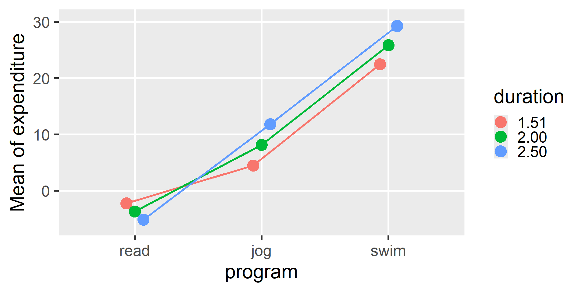
Plotting the interaction
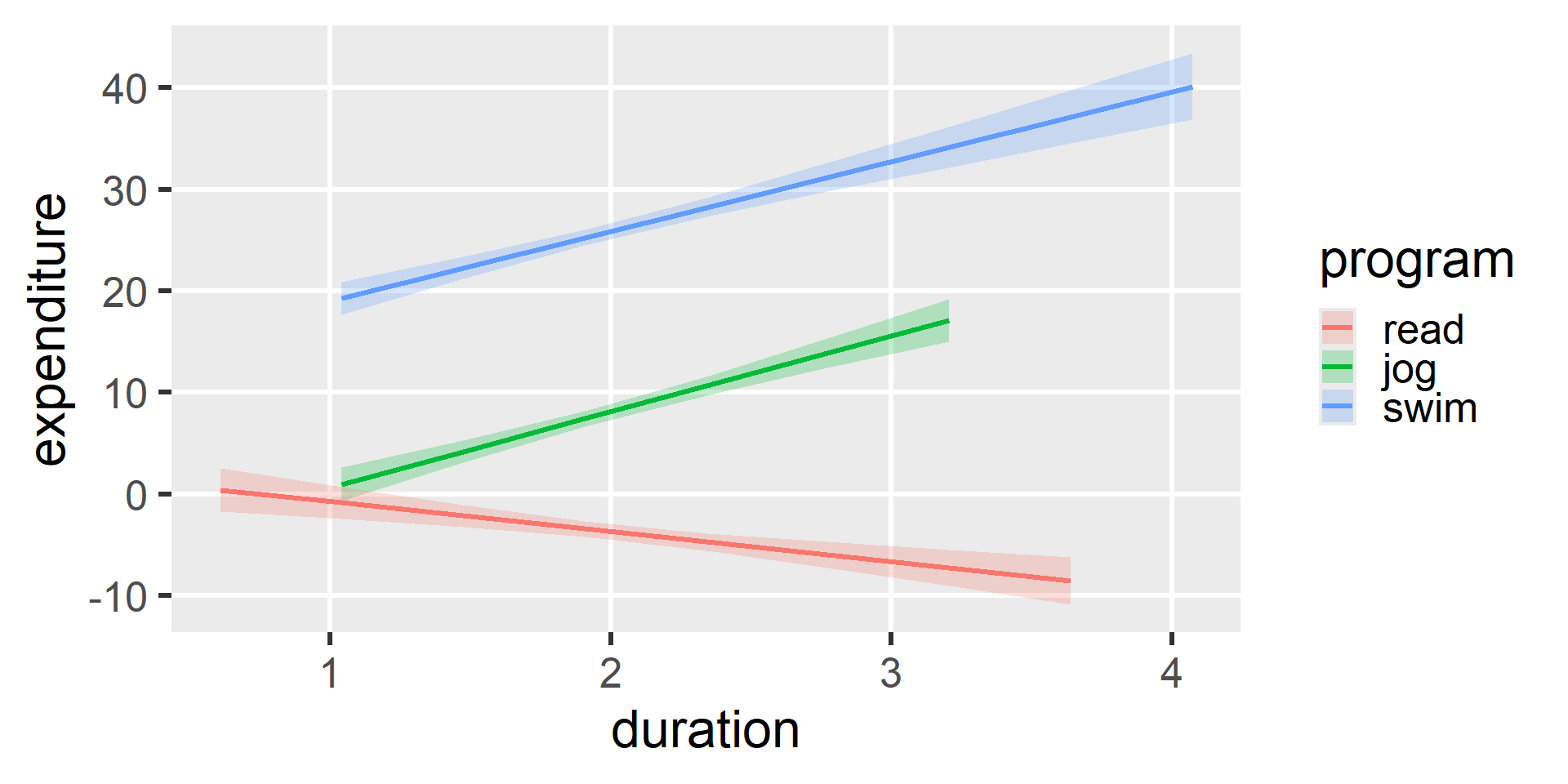
Plotting the interaction
Centering
- Do we really care about effects at zero duration?
- If not, the simple effects’ tests are not interesting
- We may prefer to center
durationinstead- Now the simple effects’ tests are at the average duration
fit4 <- lm(expenditure ~ center(duration) * program, data = exercise)
model_parameters(fit4)
## Parameter                         | Coefficient |   SE |         95% CI | t(894) |      p
## -----------------------------------------------------------------------------------------
## (Intercept)                       |       -3.70 | 0.38 | [-4.44, -2.97] |  -9.85 | < .001
## center(duration)                  |       -2.96 | 0.71 | [-4.35, -1.57] |  -4.18 | < .001
## program [jog]                     |       11.85 | 0.53 | [10.80, 12.89] |  22.29 | < .001
## program [swim]                    |       29.62 | 0.53 | [28.57, 30.66] |  55.73 | < .001
## center(duration) × program [jog]  |       10.41 | 1.07 | [ 8.30, 12.51] |   9.71 | < .001
## center(duration) × program [swim] |        9.83 | 1.05 | [ 7.77, 11.89] |   9.35 | < .001
Probing the interaction
estimate_slopes(fit4, trend = "duration", by = "program")
## Estimated Marginal Effects
##
## program | Slope |   SE |         95% CI | t(894) |      p
## ---------------------------------------------------------
## read    | -2.96 | 0.71 | [-4.35, -1.57] |  -4.18 | < .001
## jog     |  7.45 | 0.81 | [ 5.87,  9.03] |   9.25 | < .001
## swim    |  6.87 | 0.78 | [ 5.35,  8.40] |   8.84 | < .001
##
## Marginal effects estimated for duration
## Type of slope was dY/dX
Probing the interaction
estimate_contrasts(fit4, contrast = "program", by = "duration = [sd]",
                   p_adjust = "holm")
## Marginal Contrasts Analysis
##
## Level1 | Level2 | duration | Difference |   SE |         95% CI | t(894) |      p
## ---------------------------------------------------------------------------------
## jog    | read   |     1.51 |       6.70 | 0.75 | [ 5.22,  8.18] |   8.89 | < .001
## swim   | read   |     1.51 |      24.76 | 0.75 | [23.29, 26.22] |  33.12 | < .001
## swim   | jog    |     1.51 |      18.06 | 0.76 | [16.57, 19.54] |  23.91 | < .001
## jog    | read   |     2.00 |      11.84 | 0.53 | [10.80, 12.88] |  22.28 | < .001
## swim   | read   |     2.00 |      29.61 | 0.53 | [28.57, 30.66] |  55.73 | < .001
## swim   | jog    |     2.00 |      17.77 | 0.53 | [16.73, 18.81] |  33.46 | < .001
## jog    | read   |     2.50 |      16.99 | 0.75 | [15.53, 18.46] |  22.73 | < .001
## swim   | read   |     2.50 |      34.48 | 0.74 | [33.03, 35.93] |  46.63 | < .001
## swim   | jog    |     2.50 |      17.48 | 0.78 | [15.96, 19.01] |  22.45 | < .001
##
## Variable predicted: expenditure
## Predictors contrasted: program
## p-value adjustment method: Holm (1979)
Categorical-by-Categorical
Expanding the equation
We can also interact two categorical variables
We need two sets of dummy codes (e.g., [c_1] and [d_1,d_2])
\hat{y} = b_0 + b_1 c_1 + b_2 d_1 + b_3 d_2 + b_4 c_1 d_1 + b_5 c_1 d_2
expenditure ~ sex + program + sex:program
Simple and interaction effects
fit5 <- lm(expenditure ~ sex * program, data = exercise)
model_parameters(fit5)
## Parameter                   | Coefficient |   SE |         95% CI | t(894) |      p
## -----------------------------------------------------------------------------------
## (Intercept)                 |       -3.62 | 0.53 | [-4.66, -2.58] |  -6.80 | < .001
## sex [male]                  |       -0.34 | 0.75 | [-1.81,  1.14] |  -0.45 | 0.656
## program [jog]               |        7.91 | 0.75 | [ 6.43,  9.39] |  10.51 | < .001
## program [swim]              |       32.74 | 0.75 | [31.26, 34.22] |  43.49 | < .001
## sex [male] × program [jog]  |        7.82 | 1.06 | [ 5.73,  9.91] |   7.35 | < .001
## sex [male] × program [swim] | -6.26 | 1.06 | [-8.35, -4.17] | -5.88 | < .001- Intercept: estimates expenditure for females in read
- Male: male – female in read
- Jog: jog – read for females
- Swim: swim – read for females
- Male x Jog: (male – female in jog) minus (male – female in read)
- Male x Swim: (male – female in swim) minus (male – female in read)
Interaction terms are differences of differences: equivalently, Male x Jog is (jog – read for males) minus (jog – read for females)
Estimating means
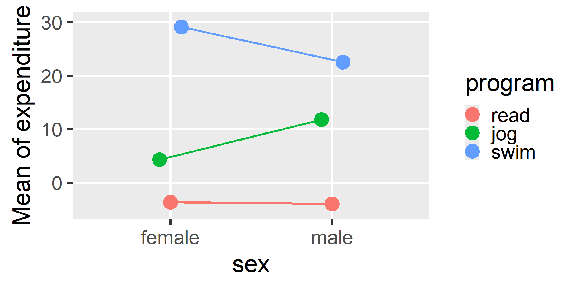
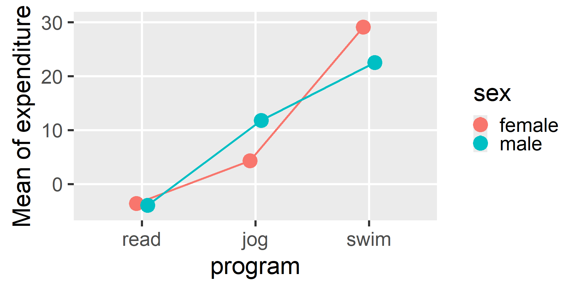
estimate_means(fit5, by = c("sex", "program"))
## Estimated Marginal Means
##
## sex    | program |  Mean |   SE |         95% CI | t(894)
## ---------------------------------------------------------
## female | read    | -3.62 | 0.53 | [-4.66, -2.58] |  -6.80
## male   | read    | -3.96 | 0.53 | [-5.00, -2.91] |  -7.43
## female | jog     |  4.29 | 0.53 | [ 3.24,  5.33] |   8.06
## male   | jog     | 11.77 | 0.53 | [10.73, 12.82] |  22.12
## female | swim    | 29.12 | 0.53 | [28.07, 30.16] |  54.71
## male   | swim    | 22.52 | 0.53 | [21.48, 23.57] |  42.32
##
## Variable predicted: expenditure
## Predictors modulated: sex, program
Estimating contrasts
estimate_contrasts(fit5, contrast = "sex", by = "program")
## Marginal Contrasts Analysis
##
## Level1 | Level2 | program | Difference |   SE |         95% CI | t(894) |      p
## --------------------------------------------------------------------------------
## male   | female | read    |      -0.34 | 0.75 | [-1.81,  1.14] |  -0.45 |  0.656
## male   | female | jog     |       7.48 | 0.75 | [ 6.01,  8.96] |   9.94 | < .001
## male   | female | swim    |      -6.60 | 0.75 | [-8.07, -5.12] |  -8.76 | < .001
##
## Variable predicted: expenditure
## Predictors contrasted: sex
## p-values are uncorrected.
Estimating contrasts
estimate_contrasts(fit5, contrast = "program", by = "sex")
## Marginal Contrasts Analysis
##
## Level1 | Level2 | sex    | Difference |   SE |         95% CI | t(894) |      p
## -------------------------------------------------------------------------------
## jog    | read   | female |       7.91 | 0.75 | [ 6.43,  9.39] |  10.51 | < .001
## swim   | read   | female |      32.74 | 0.75 | [31.26, 34.22] |  43.49 | < .001
## swim   | jog    | female |      24.83 | 0.75 | [23.35, 26.31] |  32.99 | < .001
## jog    | read   | male   |      15.73 | 0.75 | [14.25, 17.20] |  20.89 | < .001
## swim   | read   | male   |      26.48 | 0.75 | [25.00, 27.96] |  35.18 | < .001
## swim   | jog    | male   |      10.75 | 0.75 | [ 9.27, 12.23] |  14.28 | < .001
##
## Variable predicted: expenditure
## Predictors contrasted: program
## p-values are uncorrected.
Plotting the interaction
Plotting the interaction
Three-Way Interactions
When two-way isn’t enough
- So far, one moderator per effect
- Interactions can depend on a third x
- Does the sex-by-program difference hold at every exercise duration?
- Maybe it only holds in long sessions
- A three-way interaction
- Moderation of a moderation
Expanding the equation
With three predictors, every combination gets a term
For a continuous x and two dummy codes c_1 and d_1:
\hat{y} = b_0 + b_1 x + b_2 c_1 + b_3 d_1 + b_4 x c_1 + b_5 x d_1 + b_6 c_1 d_1 + b_7 x c_1 d_1
- 3 main effects, 3 two-way terms, 1 three-way term
expenditure ~ duration * sex * program
Fitting the model
fit6 <- lm(expenditure ~ duration * sex * program, data = exercise)
model_parameters(fit6)
## Parameter                                | Coefficient |   SE |           95% CI | t(888) |      p
## --------------------------------------------------------------------------------------------------
## (Intercept)                              |        0.88 | 1.80 | [ -2.64,   4.41] |   0.49 | 0.623
## duration                                 |       -2.24 | 0.86 | [ -3.93,  -0.55] |  -2.60 | 0.009
## sex [male]                               |        2.92 | 2.67 | [ -2.33,   8.16] |   1.09 | 0.275
## program [jog]                            |      -15.81 | 2.76 | [-21.23, -10.39] |  -5.73 | < .001
## program [swim]                           |       19.51 | 2.71 | [ 14.20,  24.83] |   7.20 | < .001
## duration × sex [male]                    |       -1.54 | 1.27 | [ -4.03,   0.96] |  -1.21 | 0.227
## duration × program [jog]                 |       12.06 | 1.35 | [  9.40,  14.71] |   8.91 | < .001
## duration × program [swim]                |        6.60 | 1.31 | [  4.03,   9.17] |   5.04 | < .001
## sex [male] × program [jog]               |       14.98 | 3.98 | [  7.18,  22.79] |   3.77 | < .001
## sex [male] × program [swim]              |      -18.70 | 3.90 | [-26.36, -11.04] |  -4.79 | < .001
## (duration × sex [male]) × program [jog]  |       -3.91 | 1.92 | [ -7.69,  -0.14] |  -2.03 | 0.042
## (duration × sex [male]) × program [swim] |        6.23 | 1.88 | [  2.54,   9.93] |   3.31 | < .001
Reading the output
- The coefficient table gets long fast (3 predictors gives 12 terms here)
- Read it top-down, highest-order term first
- A significant three-way term makes the two-way terms conditional
- Each lower-order term is now conditional on the others being zero
- In practice, don’t interpret this table coefficient-by-coefficient
- Probe it with estimated slopes and contrasts instead
Probing: slopes by both moderators
estimate_slopes(fit6, trend = "duration", by = c("sex", "program"))
## Estimated Marginal Effects
##
## sex    | program | Slope |   SE |         95% CI | t(888) |      p
## ------------------------------------------------------------------
## female | read    | -2.24 | 0.86 | [-3.93, -0.55] |  -2.60 |  0.009
## male   | read    | -3.78 | 0.93 | [-5.61, -1.94] |  -4.04 | < .001
## female | jog     |  9.81 | 1.04 | [ 7.77, 11.86] |   9.41 | < .001
## male   | jog     |  4.36 | 1.00 | [ 2.40,  6.33] |   4.37 | < .001
## female | swim    |  4.36 | 0.99 | [ 2.42,  6.30] |   4.42 | < .001
## male   | swim    |  9.06 | 0.98 | [ 7.13, 10.98] |   9.24 | < .001
##
## Marginal effects estimated for duration
## Type of slope was dY/dX- One duration slope per sex-by-program cell
Does the sex gap shift with duration?
estimate_contrasts(fit6, contrast = "sex", by = c("program", "duration = [sd]"),
                   p_adjust = "holm")
## Marginal Contrasts Analysis
##
## Level1 | Level2 | program | duration | Difference |   SE |          95% CI | t(888) |      p
## --------------------------------------------------------------------------------------------
## male   | female | read    |     1.51 |       0.60 | 0.95 | [ -1.26,  2.46] |   0.63 | > .999
## male   | female | jog     |     1.51 |       9.68 | 0.96 | [  7.79, 11.57] |  10.04 | < .001
## male   | female | swim    |     1.51 |      -8.71 | 0.95 | [-10.57, -6.85] |  -9.19 | < .001
## male   | female | read    |     2.00 |      -0.16 | 0.67 | [ -1.48,  1.16] |  -0.24 | > .999
## male   | female | jog     |     2.00 |       6.99 | 0.67 | [  5.67,  8.31] |  10.38 | < .001
## male   | female | swim    |     2.00 |      -6.39 | 0.67 | [ -7.70, -5.07] |  -9.51 | < .001
## male   | female | read    |     2.50 |      -0.92 | 0.89 | [ -2.68,  0.83] |  -1.03 |  0.907
## male   | female | jog     |     2.50 |       4.29 | 1.00 | [  2.33,  6.25] |   4.29 | < .001
## male   | female | swim    |     2.50 |      -4.06 | 0.97 | [ -5.98, -2.15] |  -4.17 | < .001
##
## Variable predicted: expenditure
## Predictors contrasted: sex
## p-value adjustment method: Holm (1979)
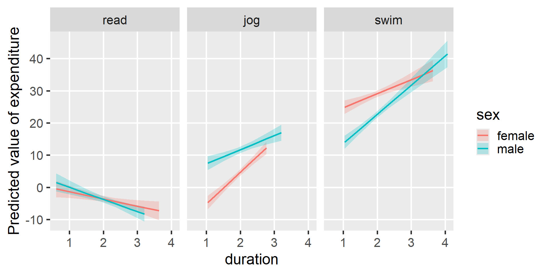
Plotting the interaction
Proceed with caution
- Three-way interactions are expensive
- They need far more power than two-way terms
- Cells get small quickly once you cross three variables
- Our example is simulated, with 150 per cell; real data is rarely this generous
- They are also easy to over-read
- A three-way term found post hoc is a HARKing risk
- Prefer to predict them in advance and preregister
- If you fit one, plot it – the coefficient table alone will rarely tell you what is going on