#install.packages("marginaleffects")
library(tidyverse)
exercise <- read_csv("exercise.csv")
exercise
## # A tibble: 900 × 6
##       id expenditure duration intensity sex   program
##    <dbl>       <dbl>    <dbl>     <dbl> <chr> <chr>
##  1     1       18.0      1.84      37.7 male  jog
##  2     2       10.2      2.39      26.7 male  jog
##  3     3       19.7      2.36      36.3 male  jog
##  4     4        1.88     2.52      20.7 male  jog
##  5     5       14.2      1.89      24.7 male  jog
##  6     6       19.7      2.37      33.7 male  jog
##  7     7       11.7      1.95      31.4 male  jog
##  8     8       22.0      2.21      39.7 male  jog
##  9     9        8.18     2.51      27.6 male  jog
## 10    10        5.03     2.17      19.2 male  jog
## # ℹ 890 more rowsStatistical Methods with R
Continuous Moderation
Unit C · Chapter 08 · Lecture 08a
Developed by Jeffrey M. Girard
Roadmap: Moderation
Overview
Continuous-by-Continuous
Interaction Patterns
Centering with Interactions
Overview
Motivation
Last chapter, we learned about multiple regression
We used this to predict y from multiple x variables
We accounted for the shared variance among x variables
We will now learn moderation (i.e., interaction effects)
The effect of one x depends on the value of another x
This adds complexity and “contextualization” to models
Example dataset
Imagine we are doing a study on exercise and energy use
Exploratory analysis
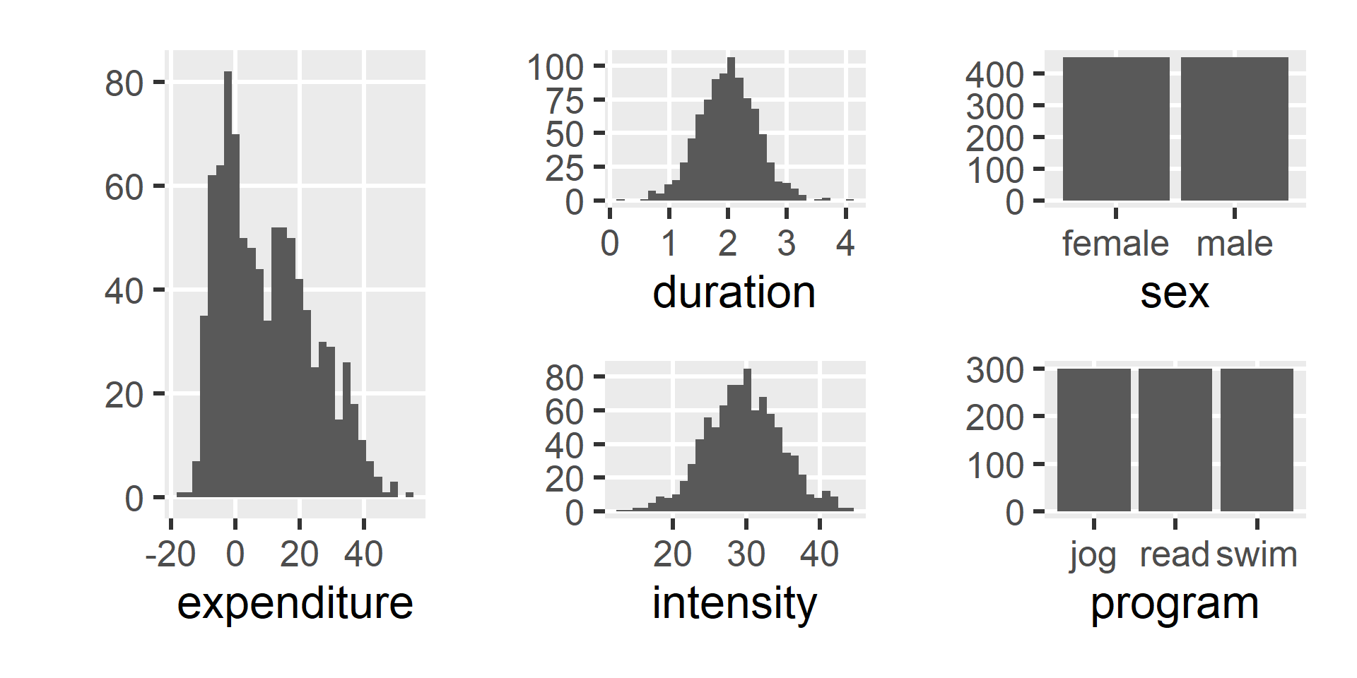
Note that this is simulated (i.e., fake) data.
Moderation questions
Continuous-by-Continuous Interaction
- Does the effect of
durationonexpendituredepend onintensity?
Continuous-by-Categorical Interaction
- Does the effect of
durationonexpendituredepend onsex?
Categorical-by-Categorical Interaction
- Does the effect of
programonexpendituredepend onsex?
Note that each question is statistically identical to its reverse (i.e., vice versa).
Continuous-by-Continuous
Multiple regression recap
Let’s regress a continuous y on two continuous x variables
\hat{y} = b_0 + b_1 x_1 + b_2 x_2
b_0 (intercept): the predicted y when x_1=0 and x_2=0
b_1 (partial): the change in y for a change of +1 in x_1
b_2 (partial): the change in y for a change of +1 in x_2
b_1 controls for x_2 but is the same across all values of x_2 and thus does not depend on it (and the same for b_2 and x_1)
Adding an interaction
Interactions are formed by multiplying predictor variables
The product becomes another predictor with its own slope
\hat{y} = b_0 + b_1 x_1 + b_2 x_2 + b_3 \color{red}{x_1 x_2}
b_0 (intercept): the predicted y when x_1=0 and x_2=0
b_1 (simple): the change in y for a change of +1 in x_1 (specifically at x_2=0)
b_2 (simple): the change in y for a change of +1 in x_2 (specifically at x_1=0)
b_3 (interaction): two equivalent definitions
- the change in b_1 (i.e., the slope of x_1) for a change of +1 in x_2
- the change in b_2 (i.e., the slope of x_2) for a change of +1 in x_1
Rearranging the formula
\hat{y} = b_0 + b_1 x_1 + b_2 x_2 + b_3 x_1 x_2
\hat{y} = b_0 + (b_1 + b_3 x_2) x_1 + b_2 x_2
Thus, the slope of x_1 (its multiplier) depends on the value of x_2
Also, if there is no interaction (b_3=0), then b_1 is unchanged
The same is true for the slope of x_2 if we rearrange again
\hat{y} = b_0 + b_1 x_1 + (b_2 + b_3 x_1) x_2
Interaction and simple effects
fit <- lm(expenditure ~ duration + intensity + duration:intensity, data = exercise)
model_parameters(fit)
## Parameter            | Coefficient |    SE |          95% CI | t(896) |     p
## -----------------------------------------------------------------------------
## (Intercept)          |        7.80 | 11.60 | [-14.97, 30.57] |   0.67 | 0.502
## duration             |       -9.38 |  5.66 | [-20.49,  1.74] |  -1.66 | 0.098
## intensity            |       -0.08 |  0.38 | [ -0.84,  0.67] |  -0.21 | 0.835
## duration × intensity |        0.39 |  0.19 | [  0.03,  0.76] |   2.10 | 0.036
The interaction effect (duration \times intensity) is significant
Thus, the effect of
durationdoes depend onintensity
We can also use the shortcut duration * intensity
Predicting energy expenditure
\hat{y} = 7.80 - 9.38 x_1 - 0.08 x_2 + 0.39 x_1 x_2
Intercept: At 0 duration and 0 intensity, a participant expends 7.8 units
Duration Simple Effect: -9.38 units per duration unit (at 0 intensity)
Intensity Simple Effect: -0.08 units per intensity unit (at 0 duration)
Interaction Effect: Each slope rises 0.39 per unit of the other
The average participant (2 duration, 30 intensity) expends 10.04 units of energy
\hat{y} = 7.80 - 9.38(2) - 0.08(30) + 0.39(2)(30) = 10.04
Spotlight analysis
In order to plot the predictions, we can map one predictor to the x-axis
But representing the other predictor continuously is challenging in 2D
- Instead of trying to use a 3D plot, we usually “spotlight” a few values, e.g.,
- One SD below the mean (\bar{x} - s_x)
- The mean value (\bar{x})
- One SD above the mean (\bar{x} + s_x)
- We plot the effect of one x on y conditional on these values of the other x
- Thus, these are often called “conditional effects plots”
- You can think of “conditional on” as “depending on”
Plotting interaction effects
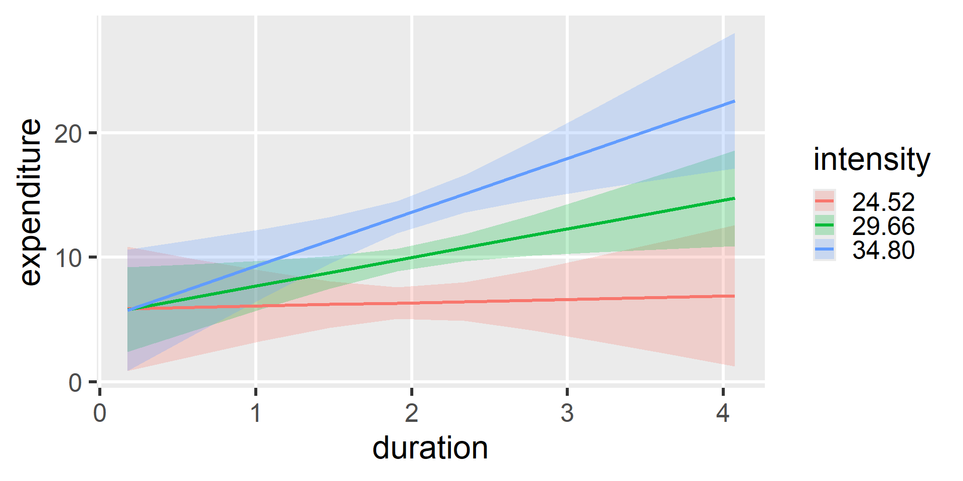
The =[sd] shortcut spotlights intensity at Mean \pm SD. The lines aren’t parallel, so the interaction is non-zero.
Plotting interaction effects
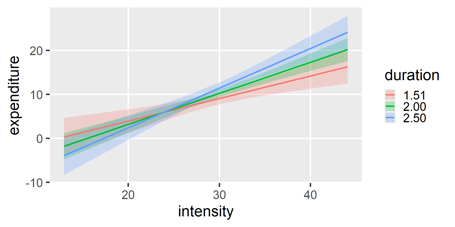
You can tell there is a non-zero interaction because the lines aren’t parallel.
Simple slopes
- What is the slope of
durationat different values ofintensity?- With a non-zero interaction, the simple slopes will differ
estimate_slopes(fit, trend = "duration", by = "intensity=c(0,15,30,45,60)")
## Estimated Marginal Effects
##
## intensity | Slope |   SE |          95% CI | t(896) |     p
## -----------------------------------------------------------
## 0         | -9.38 | 5.66 | [-20.49,  1.74] |  -1.66 | 0.098
## 15        | -3.48 | 2.92 | [ -9.21,  2.26] |  -1.19 | 0.235
## 30        |  2.42 | 0.92 | [  0.63,  4.22] |   2.65 | 0.008
## 45        |  8.32 | 2.99 | [  2.45, 14.20] |   2.78 | 0.005
## 60        | 14.23 | 5.73 | [  2.97, 25.48] |   2.48 | 0.013
##
## Marginal effects estimated for duration
## Type of slope was dY/dX
We could also use the shortcut "intensity=[sd]" to specify Mean \pm SD
Contrast with No Interaction
fit2 <- lm(expenditure ~ duration + intensity, data = exercise)
model_parameters(fit2)
## Parameter   | Coefficient |   SE |          95% CI | t(897) |      p
## --------------------------------------------------------------------
## (Intercept) |      -15.60 | 3.20 | [-21.88, -9.32] |  -4.87 | < .001
## duration    |        2.35 | 0.92 | [  0.55,  4.15] |   2.56 | 0.010
## intensity | 0.71 | 0.09 | [ 0.53, 0.88] | 8.00 | < .001- A participant exercising at 0 duration and 0 intensity expends -15.6 units
- Each additional unit of duration will expend 2.35 units (controlling
intensity) - Each additional unit of intensity will expend 0.71 units (controlling
duration) - The model predicts the same effect of duration at all values of intensity
- The model predicts the same effect of intensity at all values of duration
Plotting partial effects
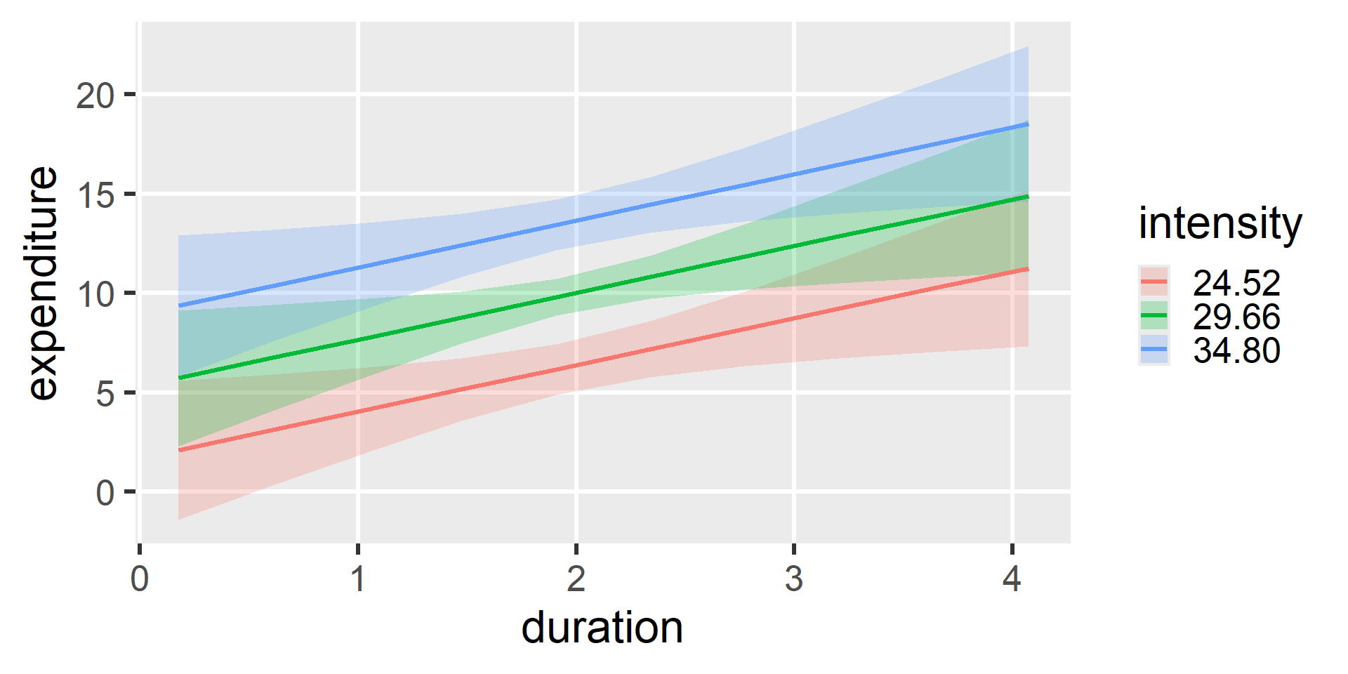
You can tell there is no interaction because the lines are parallel.
Plotting partial effects
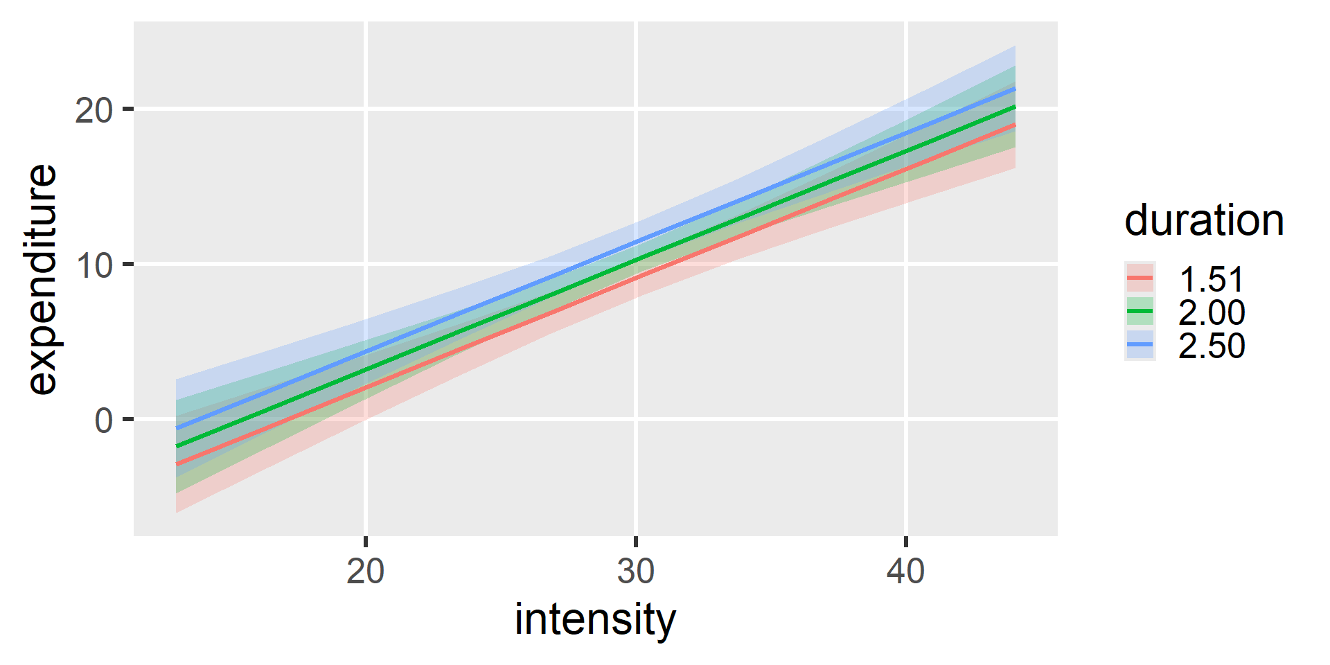
You can tell there is no interaction because the lines are parallel.
Simple slopes
- In a model with no interaction, all simple slopes are equal
estimate_slopes(fit2, trend = "duration", by = "intensity=[sd]")
## Estimated Marginal Effects
##
## intensity | Slope |   SE |       95% CI | t(897) |     p
## --------------------------------------------------------
## 24.52     |  2.35 | 0.92 | [0.55, 4.15] |   2.56 | 0.010
## 29.66     |  2.35 | 0.92 | [0.55, 4.15] |   2.56 | 0.010
## 34.80     |  2.35 | 0.92 | [0.55, 4.15] |   2.56 | 0.010
##
## Marginal effects estimated for duration
## Type of slope was dY/dX
Interaction Patterns
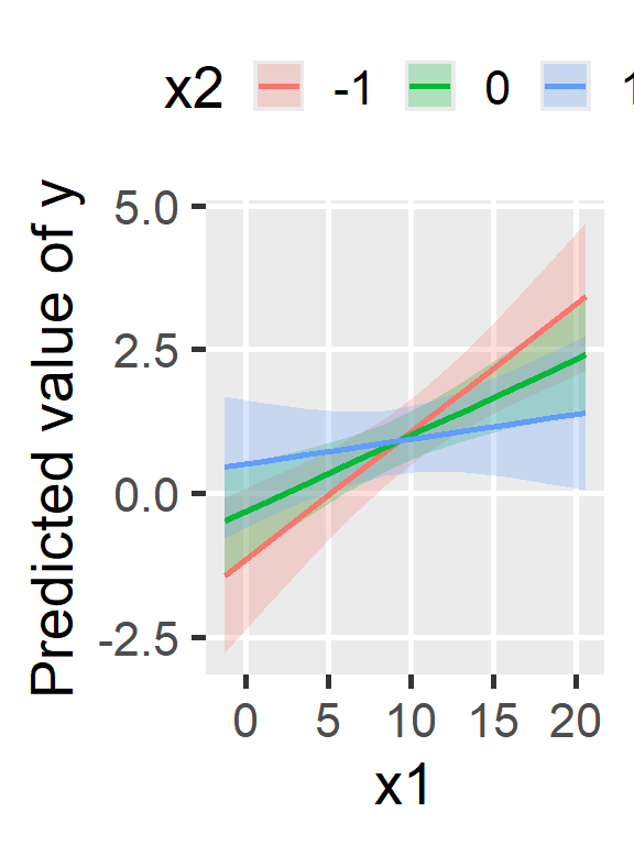
CxC Patterns
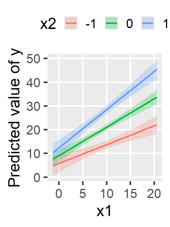
Potentiation
As one x increases, the slope of the other increases
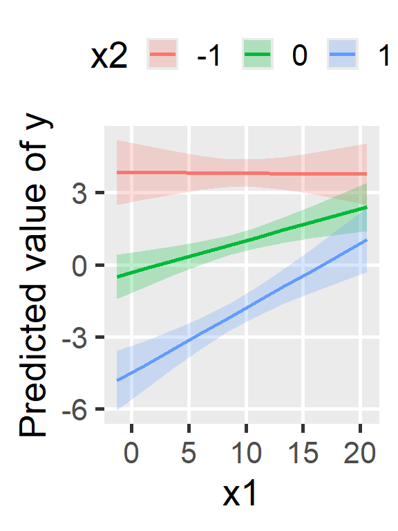
Attenuation
As one x increases, the slope of the other decreases
Crossover
As one x increases, the ranking of the other reverses
Centering with Interactions
Centering interactions
- Recall that the simple effects are when the other x=0
- This means that their p values only apply in that region
- So, if x=0 isn’t meaningful, we can use centering
- Now they are the slopes when the other x=\bar{x}
Centering interactions
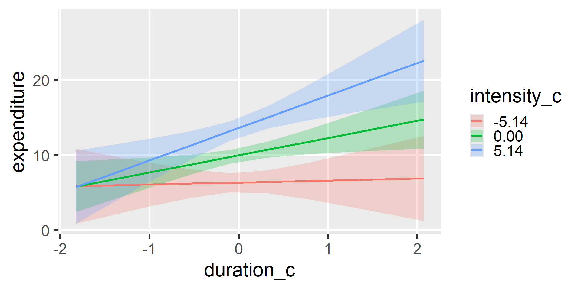
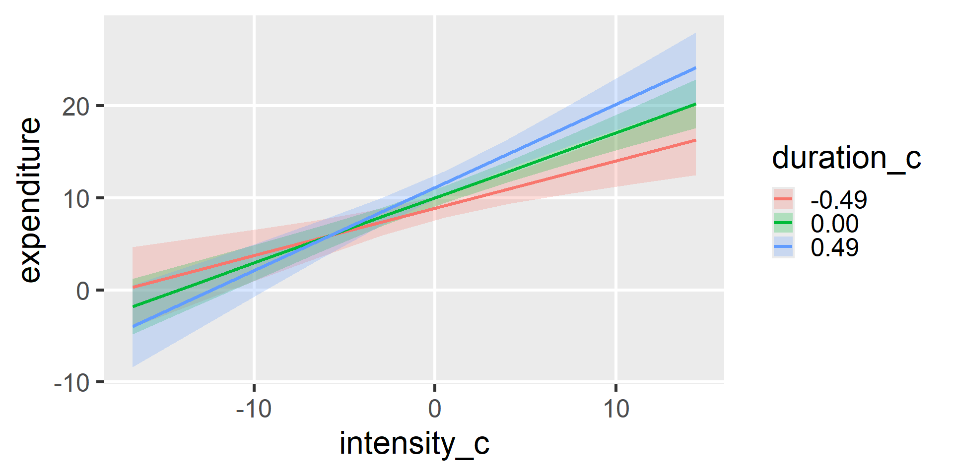
fit3 <- lm(expenditure ~ duration_c * intensity_c, data = exercise)
model_parameters(fit3)
## Parameter                | Coefficient |   SE |        95% CI | t(896) |      p
## -------------------------------------------------------------------------------
## (Intercept)              |       10.00 | 0.45 | [9.12, 10.89] |  22.13 | < .001
## duration c               |        2.29 | 0.92 | [0.49,  4.09] |   2.50 | 0.012
## intensity c              |        0.71 | 0.09 | [0.53,  0.88] |   8.04 | < .001
## duration c × intensity c |        0.39 | 0.19 | [0.03,  0.76] |   2.10 | 0.036
A participant with average duration and intensity expends 10.00 units
Each added unit of duration expends 2.29 units of energy (at average intensity)
Each added unit of intensity expends 0.71 units of energy (at average duration)
The slope of duration will increase by 0.39 for each unit of intensity, and the slope of intensity will increase by 0.39 for each unit of duration
Plotting centered interactions
Plotting centered interactions
Standardizing coefficients
- Don’t forget that standardizing includes centering!
model_parameters(fit, standardize = "refit")
## Parameter            | Coefficient |   SE |        95% CI | t(896) |      p
## ---------------------------------------------------------------------------
## (Intercept)          |   -1.15e-03 | 0.03 | [-0.06, 0.06] |  -0.04 | 0.971
## duration             |        0.08 | 0.03 | [ 0.02, 0.14] |   2.50 | 0.012
## intensity            |        0.26 | 0.03 | [ 0.20, 0.32] |   8.04 | < .001
## duration × intensity |        0.07 | 0.03 | [ 0.00, 0.14] |   2.10 | 0.036
Increasing duration by 1 SD expends another 0.08 SD (at average intensity)
Increasing intensity by 1 SD expends another 0.26 SD (at average duration)
Increasing duration by 1 SD increases the effect of intensity by 0.07 SDs and
increasing intensity by 1 SD increases the effect of duration by 0.07 SDs
Recommendations
Center your interacting continuous predictors
Use domain knowledge to guide selection of interactions
Plot your interaction effects to aid in communication
Don’t include an interaction without its simple effects
Don’t confuse simple effects and partial effects