Statistical Methods with R

Multiple Regression

Unit C · Chapter 07 · Lecture 07c

Developed by Jeffrey M. Girard

Shared Variance

Multiple regression

We often predict outcome variables using multiple predictors

  1. This will usually yield better predictions and higher \(R^2\)

  2. It will also let us isolate the predictors’ unique contributions

    • When predictors are correlated, they have redundancy
  • Example: Predict a penguin’s body mass from its bill and flipper
    • Longer bills and longer flippers both go with heavier penguins
    • However, these predictors are positively correlated
    • What is the unique contribution of each predictor?

Multiple regression

  • Let’s say we want to predict \(y\) from \(x_1\) and \(x_2\)

  • We can extend our regression equation with another slope

\[\hat{y} = b_0 + b_1x_1 + b_2x_2\]

  • \(b_1\) is related to the correlation between \(x_1\) and \(y\)

  • \(b_2\) is related to the correlation between \(x_2\) and \(y\)

  • We must account for any correlation between \(x_1\) and \(x_2\)!

Two Types of Effects

Zero-order effects

  • Fit a separate simple regression model for each predictor

\[\text{M1: }\hat{y} = b_0 + b_1x_1 \qquad\quad \text{M2: }\hat{y} = b_0 + b_1x_2\]

  • Interpretation of the \(b_1\) slope from \(\text{M1}\):
    the total relationship between \(x_1\) and \(y\) (ignoring \(x_2\))

  • Interpretation of the \(b_1\) slope from \(\text{M2}\):
    the total relationship between \(x_2\) and \(y\) (ignoring \(x_1\))

Two Types of Effects

Partial effects

  • Fit a single multiple regression model with all predictors:

\[\text{M3: }\hat{y} = b_0 + b_1x_1 + b_2x_2\]

  • Interpretation of the \(b_1\) slope from \(\text{M3}\):
    the unique relationship between \(x_1\) and \(y\) (controlling \(x_2\))
  • Interpretation of the \(b_2\) slope from \(\text{M3}\):
    the unique relationship between \(x_2\) and \(y\) (controlling \(x_1\))

Controlling predictors

  • What does it mean to statistically “control” (for) a predictor?
  • What is the relationship between \(x_1\) and \(y\) if we hold \(x_2\) at a constant value? e.g., What is the body mass difference between penguin A (40 mm bill, 190 mm flipper) and penguin B (40 mm bill, 191 mm flipper)?
  • If we already know \(x_2\), how much does learning \(x_1\) change our prediction of \(y\)? e.g., how much does learning that penguin C has a 45 mm bill change our prediction of its body mass if we already knew its flippers are 200 mm?

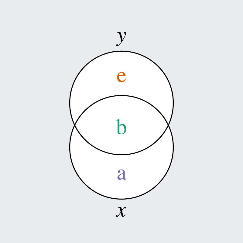
Venn diagram for simple regression

\[y_i = b_0 + b_1x_i + e_i\]

Each oval is one variable’s variance

Two oval’s overlap is their covariance

a is the variance in \(x\) unrelated to \(y\)

b is the variance shared by \(x\) and \(y\)

e is the variance in \(y\) unrelated to \(x\)

\(b_1\) represents b

\(R^2\) represents b / (b + e)

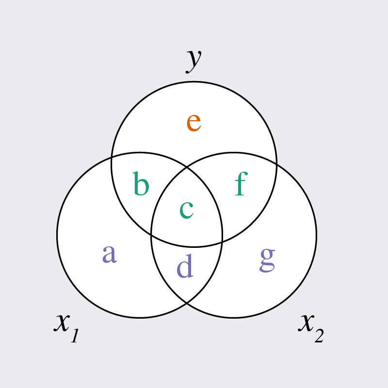
Venn diagram for two predictors

\[y_i = b_0 + b_1x_{1i} + b_2x_{2i} + e_i\]

a is the var in \(x_1\) unrelated to \(y\) or \(x_2\)

b is the var shared by \(x1\) and \(y\) (not \(x_2\))

c is the var shared by \(x_1\), \(x_2\), and \(y\)

d is the var shared by \(x_1\) and \(x_2\) (not \(y\))

e is the var in \(y\) unrelated to \(x_1\) or \(x_2\)

f is the var shared by \(x_2\) and \(y\) (not \(x_1\))

g is the var in \(x_2\) unrelated to \(x_1\) or \(y\)

Zero-order effect of \(x_1\)

\[y_i = b_0 + b_1x_{1i} + e_i\]

If we regress \(y\) on \(x_1\) only, we get the zero-order (i.e., total) effect of \(x_1\)

\(b_1\) represents b + c

\(e_i\) represents e + f

\(R^2\) represents (b + c) / (b + c + e + f)

Zero-order effect of \(x_2\)

\[y_i = b_0 + b_1x_{2i} + e_i\]

If we regress \(y\) on \(x_2\) only, we get the zero-order (i.e., total) effect of \(x_2\)

\(b_1\) represents c + f

\(e_i\) represents e + b

\(R^2\) represents (c + f) / (c + f + e + b)

Partial effects of \(x_1\) and \(x_2\)

\[y_i = b_0 + b_1x_{1i} + b_2x_{2i} + e_i\]

If we regress \(y\) on both \(x_1\) and \(x_2\), we get their partial (i.e., unique) effects

\(b_1\) represents b only

\(b_2\) represents f only

\(e_i\) represents e only

\(R^2\) represents (b + c + f) / (b + c + f + e)

c is included in \(R^2\) but neither slope

Collinearity

\[y_i = b_0 + b_1x_{1i} + b_2x_{2i} + e_i\]

If \(x_1\) and \(x_2\) are highly correlated, then c will be large and b and f may be small

Small slopes may lead you to conclude that \(x_1\) and \(x_2\) are not related to \(y\)

But this isn’t quite right… it’s just that they don’t uniquely explain \(y\) (rather, it is their overlap/shared variance that does)

So check zero-order and partial effects

Multiple Regression

Standardized partial effects

  • The relationships are clearer if we start with standardized slopes first

\[\hat{y}_i^{(z)} = \beta_1x_{1i}^{(z)} + \beta_2x_{2i}^{(z)}\]

  • We want to find the \(\beta\) values that minimize the squared residuals

\[\beta_1 = \frac{r(y,x_1)-r(y,x_2)r(x_1,x_2)}{1-r(x_1,x_2)^2}\]

\[\beta_2 = \frac{r(y,x_2)-r(y,x_1)r(x_1,x_2)}{1-r(x_1,x_2)^2}\]

  • We start with the zero-order correlation we want to partialize (i.e., that between the predictor and outcome) and then remove the redundant/shared variance

Unstandardized partial effects

  • To unstandardize the partial effects, we multiply by SD ratios

\[b_1 = \beta_1\frac{s_y}{s_{x1}}\]

\[b_2 = \beta_2\frac{s_y}{s_{x2}}\]

  • To calculate the unstandardized intercept, we can do…

\[b_0 = \bar{y} - b_1\bar{x}_1 - b_2\bar{x}_2\]

Example data

library(tidyverse)
library(easystats)
penguins <- read_csv("../../data/penguins.csv")
penguins
## # A tibble: 344 × 8
##    species island    bill_len bill_dep flipper_len body_mass sex     year
##    <chr>   <chr>        <dbl>    <dbl>       <dbl>     <dbl> <chr>  <dbl>
##  1 Adelie  Torgersen     39.1     18.7         181      3750 male    2007
##  2 Adelie  Torgersen     39.5     17.4         186      3800 female  2007
##  3 Adelie  Torgersen     40.3     18           195      3250 female  2007
##  4 Adelie  Torgersen     NA       NA            NA        NA <NA>    2007
##  5 Adelie  Torgersen     36.7     19.3         193      3450 female  2007
##  6 Adelie  Torgersen     39.3     20.6         190      3650 male    2007
##  7 Adelie  Torgersen     38.9     17.8         181      3625 female  2007
##  8 Adelie  Torgersen     39.2     19.6         195      4675 male    2007
##  9 Adelie  Torgersen     34.1     18.1         193      3475 <NA>    2007
## 10 Adelie  Torgersen     42       20.2         190      4250 <NA>    2007
## # ℹ 334 more rows

Zero-order correlations

y <- penguins$body_mass
x1 <- penguins$bill_len
x2 <- penguins$flipper_len

r_y1 <- cor(y, x1)
r_y1
## [1] NA

r_y2 <- cor(y, x2)
r_y2
## [1] NA

r_12 <- cor(x1, x2)
r_12
## [1] NA

Zero-order effects

fit1 <- lm(body_mass ~ bill_len, data = penguins)
fit2 <- lm(body_mass ~ flipper_len, data = penguins)

compare_parameters(fit1, fit2)
## Parameter    |                     fit1 |                          fit2
## -----------------------------------------------------------------------
## (Intercept)  | 362.31 (-195.02, 919.64) | -5780.83 (-6382.36, -5179.30)
## bill len     |  87.42 (  74.82, 100.01) |                              
## flipper len  |                          |    49.69 (   46.70,    52.67)
## -----------------------------------------------------------------------
## Observations |                      342 |                           342

compare_parameters(fit1, fit2, standardize = "refit")
## Parameter    |                   fit1 |                   fit2
## --------------------------------------------------------------
## (Intercept)  | 3.79e-16 (-0.09, 0.09) | 1.02e-15 (-0.05, 0.05)
## bill len     |     0.60 ( 0.51, 0.68) |                       
## flipper len  |                        |     0.87 ( 0.82, 0.92)
## --------------------------------------------------------------
## Observations |                    342 |                    342

Partial effects

fit3 <- lm(body_mass ~ bill_len + flipper_len, data = penguins)

model_parameters(fit3)
## Parameter   | Coefficient |     SE |               95% CI | t(339) |      p
## ---------------------------------------------------------------------------
## (Intercept) |    -5736.90 | 307.96 | [-6342.65, -5131.15] | -18.63 | < .001
## bill len    |        6.05 |   5.18 | [   -4.14,    16.24] |   1.17 | 0.244 
## flipper len |       48.14 |   2.01 | [   44.19,    52.10] |  23.94 | < .001

model_parameters(fit3, standardize = "refit")
## Parameter   | Coefficient |   SE |        95% CI |   t(339) |      p
## --------------------------------------------------------------------
## (Intercept) |    1.00e-15 | 0.03 | [-0.05, 0.05] | 3.78e-14 | > .999
## bill len    |        0.04 | 0.04 | [-0.03, 0.11] |     1.17 | 0.244 
## flipper len |        0.84 | 0.04 | [ 0.77, 0.91] |    23.94 | < .001

Coefficient interpretation

The intercept is the estimated body mass for a penguin with a zero-millimetre bill and zero-millimetre flippers: −5736.90 g, 95% CI: [−6342.65, −5131.15]. This is of course impossible, which is exactly why the intercept is often not worth interpreting.

The partial effect of bill length was not significantly different from zero at 6.05 g. When controlling for flipper length, each additional millimetre of bill was associated with an additional −4.14 to 16.24 g.

The partial effect of flipper length was significantly different from zero at 48.14 g. Thus, when controlling for bill length, each additional millimetre of flipper was associated with an additional 44.19 to 52.10 g.

Coefficient comparison

Note that the partial effects were smaller than the zero-order effects

  • The slope for bill_len went from 87.42 (p<.001) to 6.05 (p=.244)

  • The slope for flipper_len went from 49.69 (p<.001) to 48.14 (p<.001)

This suggests that the shared variance is doing a lot of work (especially for bill_len)

  • When we remove this shared variance, the partial effects become smaller

  • This is a very common pattern for correlated predictors in a multiple regression

  • \(x_1\) and \(x_2\) are thus “partially redundant” due to their shared variance

  • However, this is not always the pattern (e.g., in suppression effects)

Explained Variance

compare_performance(fit1, fit2, fit3, metrics = "R2")
## # Comparison of Model Performance Indices
## 
## Name | Model |    R2
## --------------------
## fit1 |    lm | 0.354
## fit2 |    lm | 0.759
## fit3 |    lm | 0.760

Moving from model fit1 to fit3 (i.e., learning flipper_len) improves \(R^2\) far more \((\Delta R^2=.406)\) than moving from model fit2 to fit3 (i.e., learning bill_len) does \((\Delta R^2=.001)\).

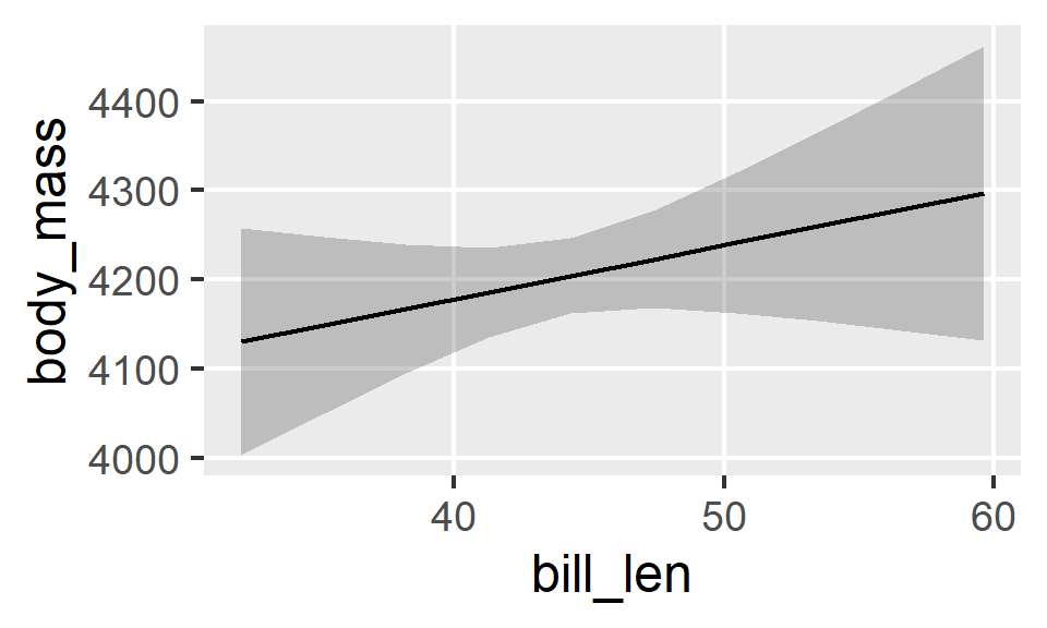
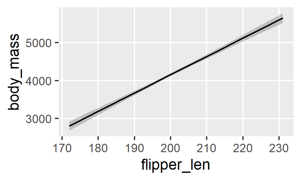
Plotting marginal effects

library(modelbased)
plot(estimate_relation(
  model = fit3,
  by = "bill_len"
))
plot(estimate_relation(
  model = fit3,
  by = "flipper_len"
))
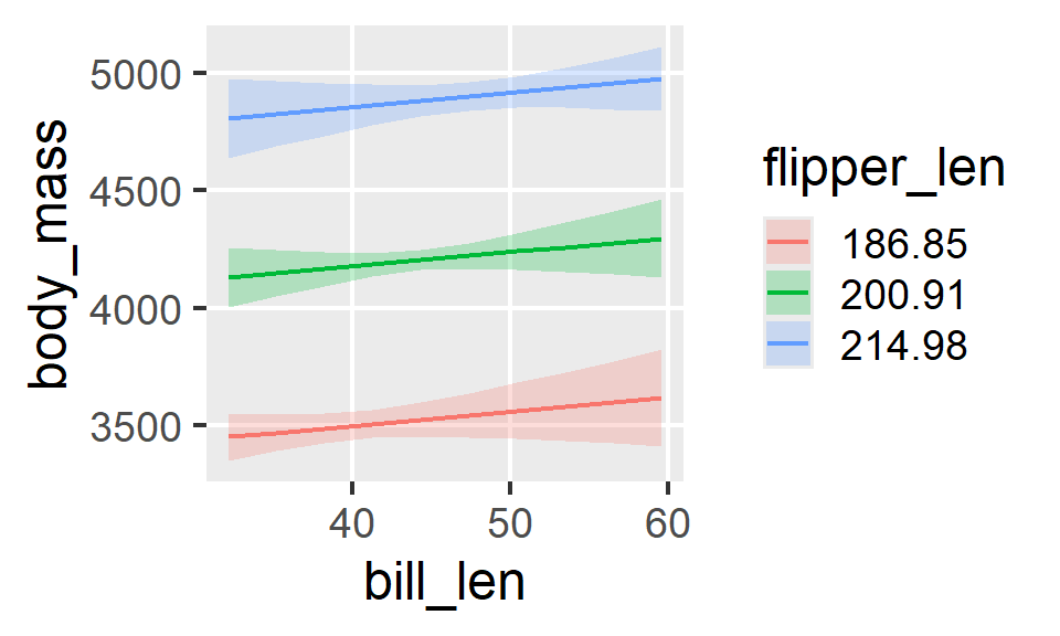
Plotting marginal effects

plot(estimate_relation(
  model = fit3,
  by = c(
    "bill_len",
    "flipper_len=[sd]"
  )
))
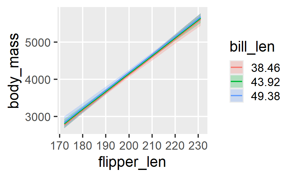
plot(estimate_relation(
  model = fit3,
  by = c(
    "flipper_len",
    "bill_len=[sd]"
  )
))
Many Predictors

Extended regression equation

  • If we have \(k\) predictors, we can add a slope for each one

\[\hat{y} = b_0 + b_1x_1 + b_2x_2 + \cdots + b_kx_k\]

  • We still find \(b\) values that minimize the squared residuals
  • The intercept is the value of \(\hat{y}\) when all predictors equal 0

  • Each slope is partial (i.e., controls for all other predictors)

  • We can combine continuous and categorical predictors!

Example zero-order effects

m_bil <- lm(body_mass ~ bill_len, data = penguins)
m_fli <- lm(body_mass ~ flipper_len, data = penguins)
m_dep <- lm(body_mass ~ bill_dep, data = penguins)
m_sex <- lm(body_mass ~ sex, data = penguins)

compare_parameters(m_bil, m_fli, m_dep, m_sex, standardize = "refit")
## Parameter    |                  m_bil |                  m_fli
## --------------------------------------------------------------
## (Intercept)  | 3.79e-16 (-0.09, 0.09) | 1.02e-15 (-0.05, 0.05)
## bill len     |     0.60 ( 0.51, 0.68) |                       
## flipper len  |                        |     0.87 ( 0.82, 0.92)
## bill dep     |                        |                       
## sex [male]   |                        |                       
## --------------------------------------------------------------
## Observations |                    342 |                    342
## 
## Parameter    |                   m_dep |                m_sex
## -------------------------------------------------------------
## (Intercept)  | 5.68e-16 (-0.09,  0.09) | -0.43 (-0.57, -0.29)
## bill len     |                         |                     
## flipper len  |                         |                     
## bill dep     |    -0.47 (-0.57, -0.38) |                     
## sex [male]   |                         |  0.85 ( 0.65,  1.04)
## -------------------------------------------------------------
## Observations |                     342 |                  333
  • All zero-order effects are significant (we can tell this from above because none of the slopes’ 95% CIs contain zero)

Example partial effects

m_all <- lm(body_mass ~ bill_len + flipper_len + bill_dep + sex, data = penguins)
model_parameters(m_all, standardize = "refit")
## Parameter   | Coefficient |   SE |         95% CI | t(328) |      p
## -------------------------------------------------------------------
## (Intercept) |       -0.34 | 0.04 | [-0.42, -0.26] |  -8.51 | < .001
## bill len    |       -0.02 | 0.03 | [-0.08,  0.05] |  -0.50 | 0.619 
## flipper len |        0.68 | 0.04 | [ 0.59,  0.76] |  15.86 | < .001
## bill dep    |       -0.21 | 0.04 | [-0.29, -0.14] |  -5.53 | < .001
## sex [male]  |        0.67 | 0.06 | [ 0.55,  0.80] |  10.46 | < .001
  • “The partial effect of flipper length was significant (p<.001). Thus, while controlling for sex and bill length and depth, each SD increase in flipper length was associated with a 0.68 SD increase in body mass.”

Example effect sizes

compare_performance(m_bil, m_fli, m_dep, m_sex, m_all, 
                    metrics = c("R2", "R2_adj"))
## # Comparison of Model Performance Indices
## 
## Name  | Model |    R2 | R2 (adj.)
## ---------------------------------
## m_bil |    lm | 0.354 |     0.352
## m_fli |    lm | 0.759 |     0.758
## m_dep |    lm | 0.223 |     0.220
## m_sex |    lm | 0.181 |     0.178
## m_all |    lm | 0.823 |     0.821
  • “The linear model predicting body mass from bill length, flipper length, bill depth, and sex explained most of the variance in body mass (R²=.823, Adjusted R²=.821).”

Striking a balance

  • Covariates are predictors we only want to control

    • The linear model does not treat them differently
  • In some fields, it is common to include many covariates

  • Relevant predictors should be included but don’t go too far

    • Adding predictors can decrease your power
    • Adding predictors can lead to collinearity
    • Adding predictors can change your interpretation
  • Think carefully about what to include vs. exclude