Statistical Methods with R

Categorical Predictors

Unit C · Chapter 07 · Lecture 07b

Developed by Jeffrey M. Girard

Introduction

Categorical variables

We learned regression with a single continuous predictor
Today we learn about regression with a categorical predictor

We use factor() to tell R that a variable is categorical
Our factor puts each observation into one of \(g\) groups

Groups must be mutually exclusive and exhaustive
- No observation is in more than one group/category
- All observations are in a group/category

Terminology and examples

Two groups: “binary” or “dichotomous”
- e.g., \(\text{Condition}\in\{\text{Control}, \text{Treatment}\}\)
- e.g., \(\text{Gender}\in\{\text{Man}, \text{Woman}\}\)
Three or more groups: “nominal” or “polytomous”
- e.g., \(\text{Nation}\in\{\text{UK}, \text{Germany}, \text{Spain}, \text{France}\}\)
- e.g., \(\text{Sect}\in\{\text{Catholic}, \text{Protestant}, \text{Orthodox}\}\)
- e.g., \(\text{Time}\in\{\text{Baseline}, \text{Midpoint}, \text{Endpoint}\}\)*

Code variables

To use factors as predictors, we need to quantify them
- We turn them into numerical code variables

There are several methods called coding systems
- Coding systems may change the code and coefficients
- But they don’t change the predictions or model fit

All coding systems turn a factor into \(g-1\) code variables
- So if we have 6 groups, we need 5 code variables

Dichotomous
Dummy Coding

Coding two categories

Dummy coding uses a value of \(0\) or \(1\) for each code variable
- With two categories, we only need one code variable: \(C_1\)
- One category gets \(C_1=0\) and the other gets \(C_1=1\)
- The category assigned to \(0\) is called the “reference group”

Female as Reference

Sex	C₁
Female*	0
Male	1

Male as Reference

Sex	C₁
Female	1
Male*	0

Example dataset

penguins <- read_csv("../../data/penguins.csv")
penguins
## # A tibble: 344 × 8
##    species island    bill_len bill_dep flipper_len body_mass sex     year
##    <chr>   <chr>        <dbl>    <dbl>       <dbl>     <dbl> <chr>  <dbl>
##  1 Adelie  Torgersen     39.1     18.7         181      3750 male    2007
##  2 Adelie  Torgersen     39.5     17.4         186      3800 female  2007
##  3 Adelie  Torgersen     40.3     18           195      3250 female  2007
##  4 Adelie  Torgersen     NA       NA            NA        NA <NA>    2007
##  5 Adelie  Torgersen     36.7     19.3         193      3450 female  2007
##  6 Adelie  Torgersen     39.3     20.6         190      3650 male    2007
##  7 Adelie  Torgersen     38.9     17.8         181      3625 female  2007
##  8 Adelie  Torgersen     39.2     19.6         195      4675 male    2007
##  9 Adelie  Torgersen     34.1     18.1         193      3475 <NA>    2007
## 10 Adelie  Torgersen     42       20.2         190      4250 <NA>    2007
## # ℹ 334 more rows

Dummy coding by hand

We can use the recode() function from {tidyverse}

penguins$sex_c1 <- recode(penguins$sex, female = 1, male = 0)
penguins
## # A tibble: 344 × 9
##    species island    bill_len bill_dep flipper_len body_mass sex     year sex_c1
##    <chr>   <chr>        <dbl>    <dbl>       <dbl>     <dbl> <chr>  <dbl>  <dbl>
##  1 Adelie  Torgersen     39.1     18.7         181      3750 male    2007      0
##  2 Adelie  Torgersen     39.5     17.4         186      3800 female  2007      1
##  3 Adelie  Torgersen     40.3     18           195      3250 female  2007      1
##  4 Adelie  Torgersen     NA       NA            NA        NA <NA>    2007     NA
##  5 Adelie  Torgersen     36.7     19.3         193      3450 female  2007      1
##  6 Adelie  Torgersen     39.3     20.6         190      3650 male    2007      0
##  7 Adelie  Torgersen     38.9     17.8         181      3625 female  2007      1
##  8 Adelie  Torgersen     39.2     19.6         195      4675 male    2007      0
##  9 Adelie  Torgersen     34.1     18.1         193      3475 <NA>    2007     NA
## 10 Adelie  Torgersen     42       20.2         190      4250 <NA>    2007     NA
## # ℹ 334 more rows

Regression with a dummy code

We can regress body_mass on the numeric dummy code \(C_1\)

\[\hat{y}_i = b_0 + b_1 C_{1i}\]

The intercept \(b_0\) is the value of \(\hat{y}\) when \(C_1=0\)
- i.e., the reference group’s average outcome value
The slope \(b_1\) is the change in \(\hat{y}\) when \(C_1+1\)
- i.e., the group difference in average outcome values

Regression with a dummy code

fit <- lm(formula = body_mass ~ sex_c1, data = penguins)
fit
## 
## Call:
## lm(formula = body_mass ~ sex_c1, data = penguins)
## 
## Coefficients:
## (Intercept)       sex_c1  
##      4545.7       -683.4

The average body mass of male penguins is 4545.68 g
Female penguins weigh 683.41 g less on average

The factor shortcut (recommended)

R will automatically generate dummy codes for factors
- It will use the first level as the reference group
- It will name the slope “factorNonref” (e.g., sexFemale)

penguins$sex <- factor(penguins$sex, levels = c("male", "female"))
fit2 <- lm(formula = body_mass ~ sex, data = penguins)
fit2
## 
## Call:
## lm(formula = body_mass ~ sex, data = penguins)
## 
## Coefficients:
## (Intercept)    sexfemale  
##      4545.7       -683.4

Swapping the reference group

To use female as the reference group, we just put it first

penguins$sex <- factor(penguins$sex, levels = c("female", "male"))
fit3 <- lm(formula = body_mass ~ sex, data = penguins)
fit3
## 
## Call:
## lm(formula = body_mass ~ sex, data = penguins)
## 
## Coefficients:
## (Intercept)      sexmale  
##      3862.3        683.4

The average body mass of female penguins is 3862.27 g
Male penguins weigh 683.41 g more on average

Parameter significance testing

Testing is the same as with a continuous predictor

model_parameters(fit2)
## Parameter    | Coefficient |    SE |             95% CI | t(331) |      p
## -------------------------------------------------------------------------
## (Intercept)  |     4545.68 | 56.32 | [4434.90, 4656.47] |  80.71 | < .001
## sex [female] |     -683.41 | 80.01 | [-840.80, -526.02] |  -8.54 | < .001

“The average body mass of female penguins was estimated to be 683.41 grams lower than that of male penguins, 95% CI: [–840.80, –526.02], t = –8.54, p < .001.”

Relation to Student’s t-test

fit2b <- t.test(body_mass ~ sex, data = penguins, var.equal = TRUE)
model_parameters(fit2b)
## Two Sample t-test
## 
## Parameter | Group | sex = female | sex = male | Difference |             95% CI
## -------------------------------------------------------------------------------
## body_mass |   sex |      3862.27 |    4545.68 |    -683.41 | [-840.80, -526.02]
## 
## Parameter | t(331) |      p
## ---------------------------
## body_mass |  -8.54 | < .001
## 
## Alternative hypothesis: true difference in means between group female and group male is not equal to 0

The slope test and Student’s t-test give the same results
- The linear model (lm) “subsumes” Student’s t-test
- It also assumes equal variances in the two groups

Effect sizes

The standardized slope is similar to Cohen’s \(d\)

model_parameters(fit2, standardize = "refit")
## Parameter    | Coefficient |   SE |         95% CI | t(331) |      p
## --------------------------------------------------------------------
## (Intercept)  |        0.42 | 0.07 | [ 0.28,  0.56] |   6.01 | < .001
## sex [female] |       -0.85 | 0.10 | [-1.04, -0.65] |  -8.54 | < .001

“The average body mass of female penguins was 0.85 standard deviations lower than that of male penguins, 95% CI: [–1.04, –0.65], p<.001.”

Effect sizes

We can also use \(R^2\) or Adjusted \(R^2\) as before

r2(fit2, ci = 0.95)
##        R2: 0.181 [0.110, 0.259]
##   adj. R2: 0.178 [0.108, 0.256]

“Around 18% of the variance in penguins’ body mass was explained by sex,
R² = .181, 95% CI: [.110, .259], Adjusted R² = .178.”

Estimating means by hand

\[ \begin{align} \text{Model Equation: }&\hat{y}=b_0 + b_1(C_1)\\ &\hat{y} = 4545.68 -683.41(C_1)\\ \\ \text{Male penguins: }&\hat{y} = 4545.68 -683.41(0)=4545.68 \\ \text{Female penguins: }&\hat{y} = 4545.68 -683.41(1)=3862.27 \end{align} \]

Each penguin \(i\) will have a residual \(e_i\) that pushes its body mass above or below the mean for its group (i.e., sex)

\[y_i=4545.68-683.41(C_1)+e_i\]

Estimating means in R

gmeans <- estimate_means(fit2, by = "sex")
gmeans
## Estimated Marginal Means
## 
## sex    |    Mean |    SE |             95% CI | t(331)
## ------------------------------------------------------
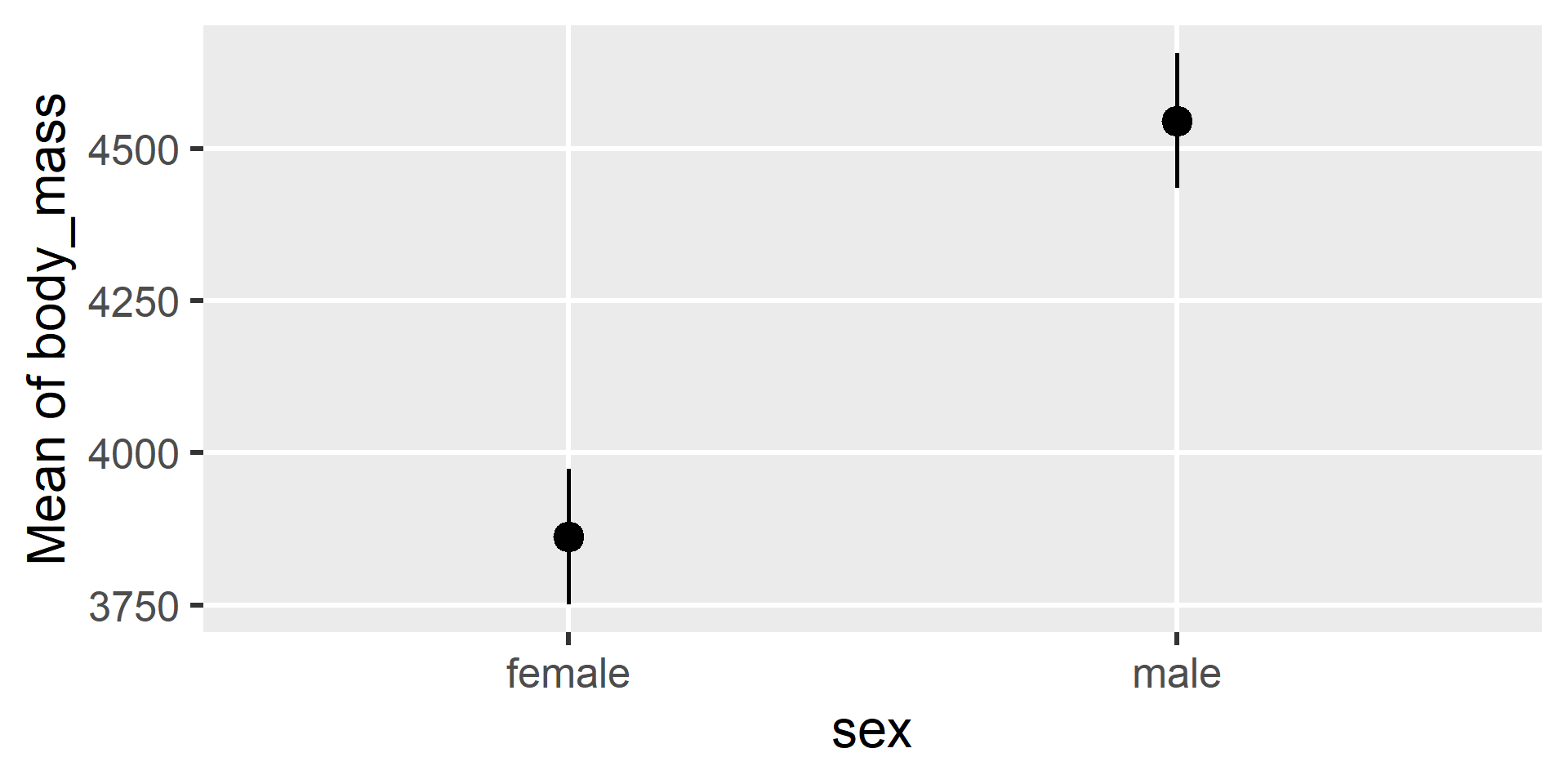
## female | 3862.27 | 56.83 | [3750.48, 3974.06] |  67.96
## male   | 4545.68 | 56.32 | [4434.90, 4656.47] |  80.71
## 
## Variable predicted: body_mass
## Predictors modulated: sex

Plotting means in R

plot(gmeans)

Polytomous
Dummy Coding

Coding many categories

With three categories, we need two code variables: \([C_1, C_2]\)
The reference group will get \(0\) on all code variables
Each other group will get \(1\) on a single code variable

Alcohol as Reference

Condition	C₁	C₂
Alcohol*	0	0
Placebo	1	0
Control	0	1

Placebo as Reference

Condition	C₁	C₂
Alcohol	1	0
Placebo*	0	0
Control	0	1

Control as Reference

Condition	C₁	C₂
Alcohol	1	0
Placebo	0	1
Control*	0	0

Selecting the reference group

The reference group has implications for interpretation

The reference group should be a useful comparison
- e.g., a control group or standard treatment
The reference group should be well-defined
- e.g., not an “other” or “wastebasket” category
The reference group should not be relatively small
- e.g., not a group of 10 when others have 100

Creating dummy codes by hand

To create the dummy codes, we can use recode() again

penguins$species_c1 <- recode(penguins$species, Adelie=0, Chinstrap=1, Gentoo=0)

penguins$species_c2 <- recode(penguins$species, Adelie=0, Chinstrap=0, Gentoo=1)

This can get tedious as the number of groups increases
It’s easier and less error-prone to use the factor shortcut

penguins$species <- factor(
  penguins$species,
  levels = c("Adelie", "Chinstrap", "Gentoo")
)

Regression with many dummy codes

To use many dummy codes, we need multiple regression
- Basically, we add another predictor and another slope

\[\hat{y} = b_0 + b_1C_1 + b_2C_2\]

The intercept \(b_0\) is the mean of the reference group
The slope \(b_1\) is the reference vs. \(C_1=1\) group difference
The slope \(b_2\) is the reference vs. \(C_2=1\) group difference

Regression with many dummy codes

fit4 <- lm(body_mass ~ species_c1 + species_c2, data = penguins)
fit4
## 
## Call:
## lm(formula = body_mass ~ species_c1 + species_c2, data = penguins)
## 
## Coefficients:
## (Intercept)   species_c1   species_c2  
##     3700.66        32.43      1375.35

Adelie species averages 3700.66 g
Chinstrap species averages 32.43 g more than Adelie species
Gentoo species averages 1375.35 g more than Adelie species

Parameter significance testing

model_parameters(fit4)
## Parameter   | Coefficient |    SE |             95% CI | t(339) |      p
## ------------------------------------------------------------------------
## (Intercept) |     3700.66 | 37.62 | [3626.67, 3774.66] |  98.37 | < .001
## species c1  |       32.43 | 67.51 | [-100.37,  165.22] |   0.48 | 0.631 
## species c2  |     1375.35 | 56.15 | [1264.91, 1485.80] |  24.50 | < .001

Intercept: Is the Adelie species body mass zero?
\(C_1\) Slope: Is the Chinstrap-Adelie group difference zero?
\(C_2\) Slope: Is the Gentoo-Adelie group difference zero?

The factor shortcut

fit5 <- lm(body_mass ~ species, data = penguins)
model_parameters(fit5)
## Parameter           | Coefficient |    SE |             95% CI | t(339) |      p
## --------------------------------------------------------------------------------
## (Intercept)         |     3700.66 | 37.62 | [3626.67, 3774.66] |  98.37 | < .001
## species [Chinstrap] |       32.43 | 67.51 | [-100.37,  165.22] |   0.48 | 0.631 
## species [Gentoo]    |     1375.35 | 56.15 | [1264.91, 1485.80] |  24.50 | < .001

Note that we already set the factor up on slide 25
The parameter table includes which level each code is for

Model significance testing

What is the overall effect of species (à la ANOVA)?
- Do all categories have the same mean?
- We can actually give the lm() results to aov()

fit5b <- aov(fit5)
model_parameters(fit5b)
## Parameter | Sum_Squares |  df | Mean_Square |      F |      p
## -------------------------------------------------------------
## species   |    1.47e+08 |   2 |    7.34e+07 | 343.63 | < .001
## Residuals |    7.24e+07 | 339 |    2.14e+05 |        |       
## 
## Anova Table (Type 1 tests)

Effect sizes

model_parameters(fit5, standardize = "refit")
## Parameter           | Coefficient |   SE |         95% CI | t(339) |      p
## ---------------------------------------------------------------------------
## (Intercept)         |       -0.62 | 0.05 | [-0.72, -0.53] | -13.32 | < .001
## species [Chinstrap] |        0.04 | 0.08 | [-0.13,  0.21] |   0.48 | 0.631 
## species [Gentoo]    |        1.72 | 0.07 | [ 1.58,  1.85] |  24.50 | < .001

r2(fit5, ci = 0.95)
##        R2: 0.670 [0.607, 0.722]
##   adj. R2: 0.668 [0.604, 0.720]

Chinstrap species averages 0.04 SDs higher body mass than Adelie
Gentoo species averages 1.72 SDs higher body mass than Adelie
Species explained 67% of the variance in body mass

Estimating means by hand

\[ \begin{align} \text{Equation: }&\hat{y} = b_0 + b_1(C_1) + b_2(C_2) \\ &\hat{y} = 3700.66 + 32.43(C_1) + 1375.35(C_2) \\ \\ \text{Adelie: } &\hat{y} = 3700.66 + 32.43(0) + 1375.35(0) = 3700.66 \\ \text{Chinstrap: }&\hat{y} = 3700.66 + 32.43(1) + 1375.35(0) = 3733.09 \\ \text{Gentoo: } &\hat{y} = 3700.66 + 32.43(0) + 1375.35(1) = 5076.01 \end{align} \]

Estimating means in R

gmeans <- estimate_means(fit5, by = "species")
gmeans
## Estimated Marginal Means
## 
## species   |    Mean |    SE |             95% CI | t(339)
## ---------------------------------------------------------
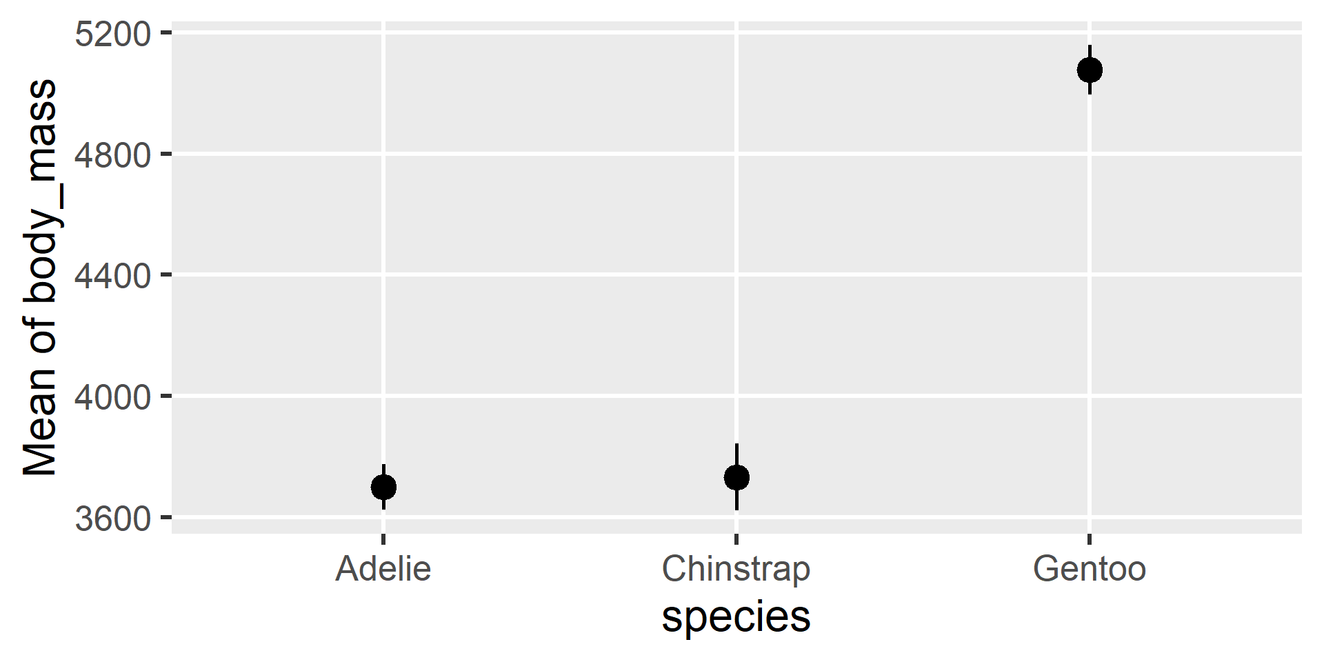
## Adelie    | 3700.66 | 37.62 | [3626.67, 3774.66] |  98.37
## Chinstrap | 3733.09 | 56.06 | [3622.82, 3843.36] |  66.59
## Gentoo    | 5076.02 | 41.68 | [4994.03, 5158.00] | 121.78
## 
## Variable predicted: body_mass
## Predictors modulated: species

Plotting means in R

plot(gmeans)

Contrasts

What about the difference between Chinstrap and Gentoo?
How can we compare non-reference groups to each other?

estimate_contrasts(fit5, contrast = "species")
## Marginal Contrasts Analysis
## 
## Level1    | Level2    | Difference |    SE |             95% CI | t(339) |      p
## ---------------------------------------------------------------------------------
## Chinstrap | Adelie    |      32.43 | 67.51 | [-100.37,  165.22] |   0.48 |  0.631
## Gentoo    | Adelie    |    1375.35 | 56.15 | [1264.91, 1485.80] |  24.50 | < .001
## Gentoo    | Chinstrap |    1342.93 | 69.86 | [1205.52, 1480.34] |  19.22 | < .001
## 
## Variable predicted: body_mass
## Predictors contrasted: species
## p-values are uncorrected.

Categorical Predictors

Introduction

Categorical variables

Terminology and examples

Code variables

Dichotomous Dummy Coding

Coding two categories

Example dataset

Dummy coding by hand

Regression with a dummy code

Regression with a dummy code

The factor shortcut (recommended)

Swapping the reference group

Parameter significance testing

Relation to Student’s t-test

Effect sizes

Effect sizes

Estimating means by hand

Estimating means in R

Plotting means in R

Polytomous Dummy Coding

Coding many categories

Selecting the reference group

Creating dummy codes by hand

Regression with many dummy codes

Regression with many dummy codes

Parameter significance testing

The factor shortcut

Model significance testing

Effect sizes

Estimating means by hand

Estimating means in R

Plotting means in R

Contrasts

Dichotomous
Dummy Coding

Polytomous
Dummy Coding