Statistical Methods with R

Simple Regression

Unit C · Chapter 07 · Lecture 07a

Developed by Jeffrey M. Girard

Introduction

Regression as Fancy Correlation

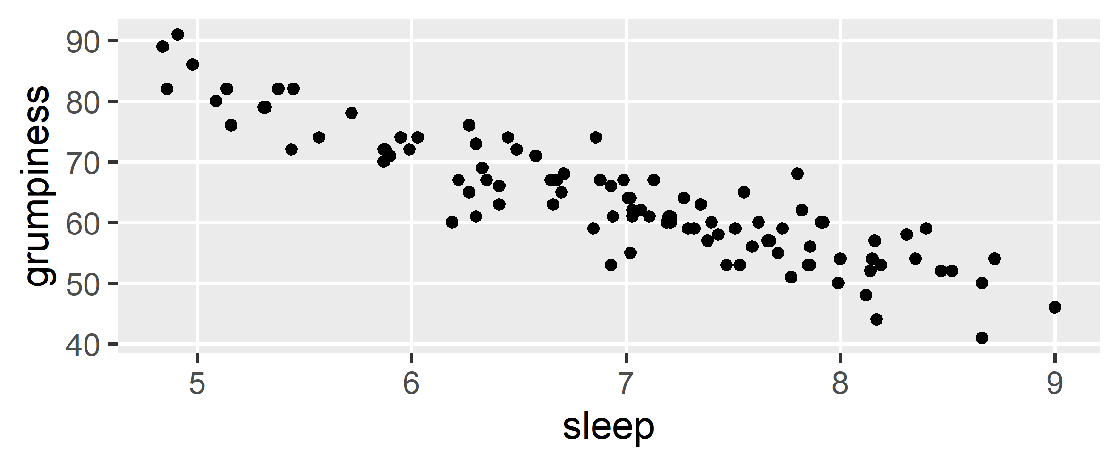
A correlation quantifies how well a straight line represents the relationship between two continuous variables

Regression as Fancy Correlation

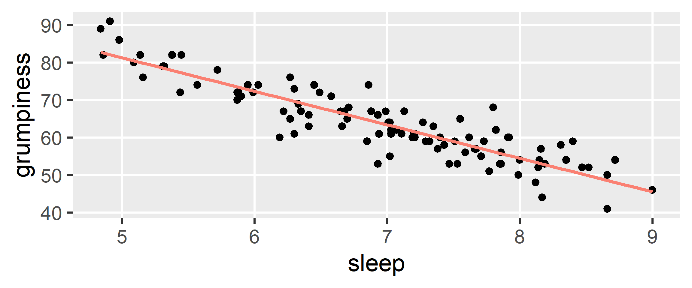
A correlation quantifies how well a straight line represents the relationship between two continuous variables

Regression as Fancy Correlation

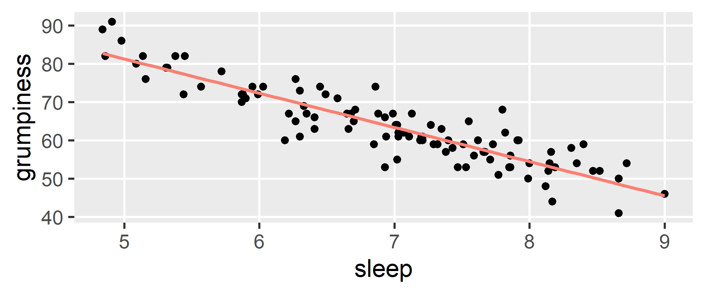
But how did we know where to draw the line?
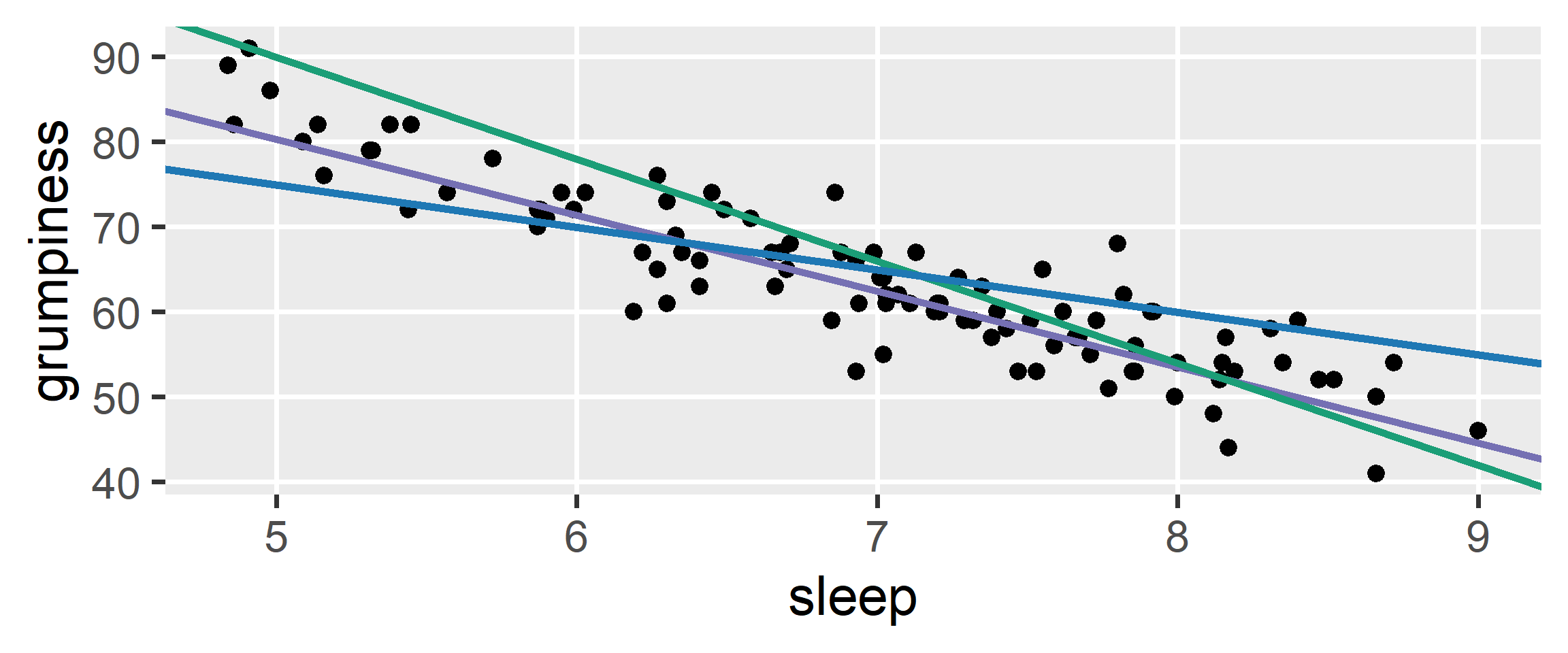
Many different lines could have been drawn…

Regression as Fancy Correlation

Regression is a way to select and quantify the “best” line

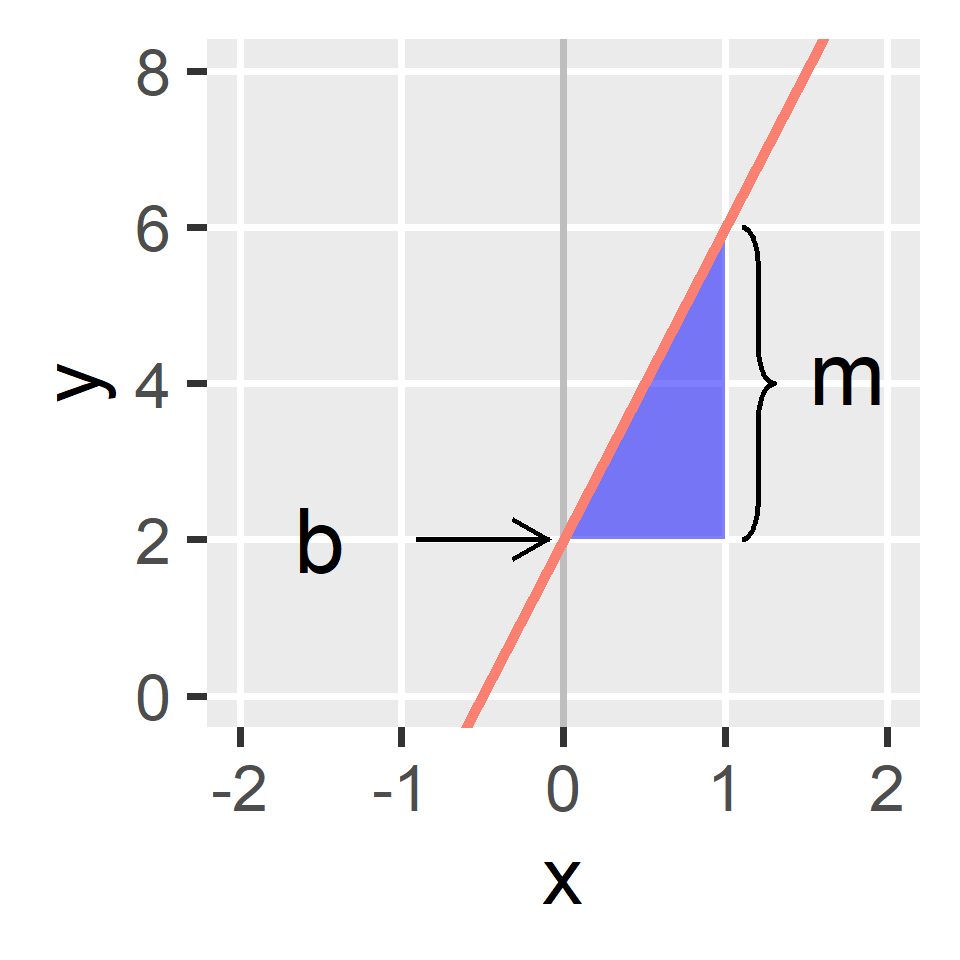
Defining a Line in General

\[y = \color{blue}{m}x + \color{blue}{b}\]

\(y\) and \(x\) are variables

\(\color{blue}m\) and \(\color{blue}b\) are coefficients

\(\color{blue}m\) is the slope
Change in \(y\) when \(x+1\)
\(\color{blue}b\) is the intercept
Value of \(y\) when \(x=0\)

Defining a Regression Line

If \(y\) is the outcome and \(x\) is the predictor…
We can define the regression line in the same way

\[\color{red}{\hat{y}_i} = \color{blue}{b_0} + \color{blue}{b_1}x_i\]

\(\color{red}{\hat{y}_i}\) is the model-predicted value of \(y\) for observation \(i\)

\(\color{blue}{b_0}\) is the intercept of the line (i.e., \(b\) on the previous slide)

\(\color{blue}{b_1}\) is the slope of the line (i.e., \(m\) on the previous slide)

Defining Regression Residuals

Our regression line is defined by the formula:

\[\color{red}{\hat{y}_i} = \color{blue}{b_0} + \color{blue}{b_1}x_i\]

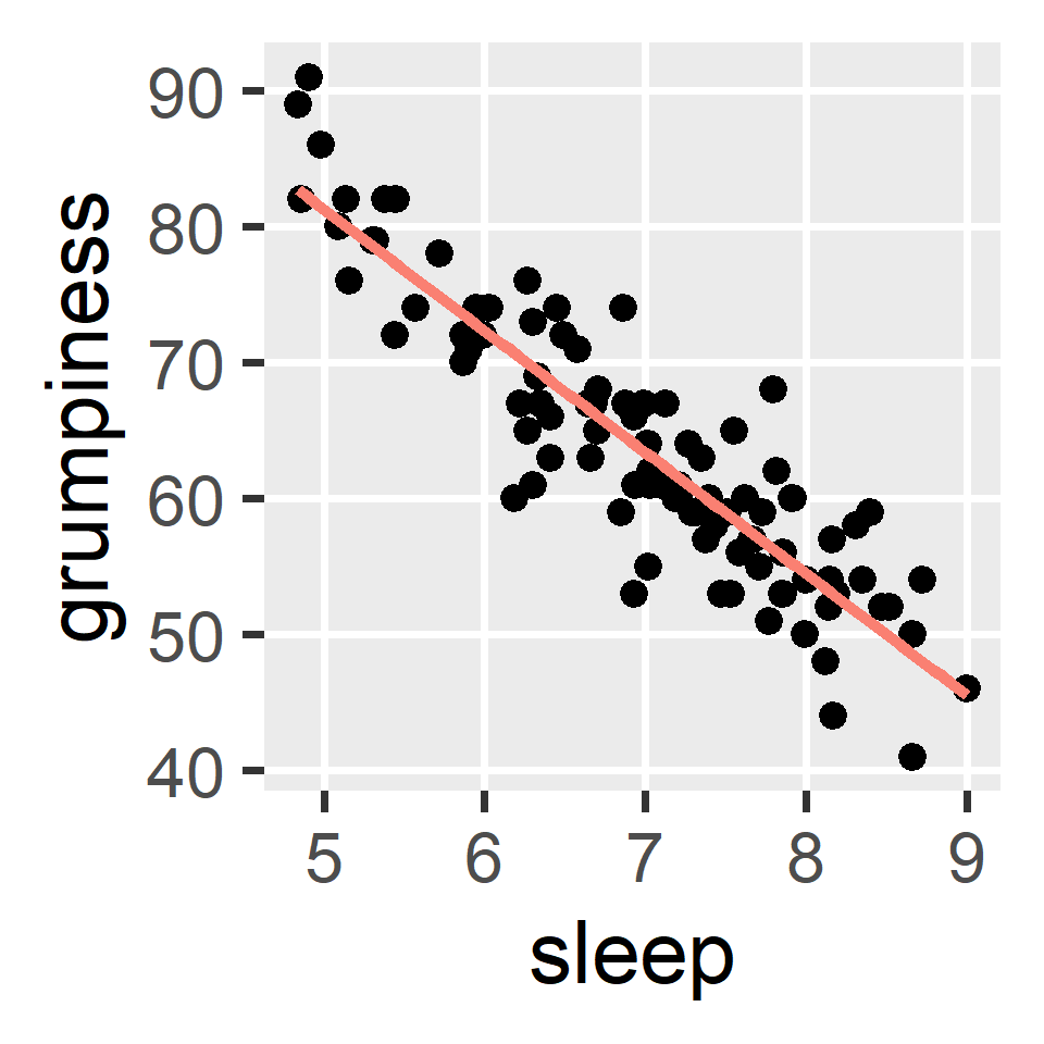
But many points aren’t exactly on the line, so our predictions aren’t perfect

Defining Regression Residuals

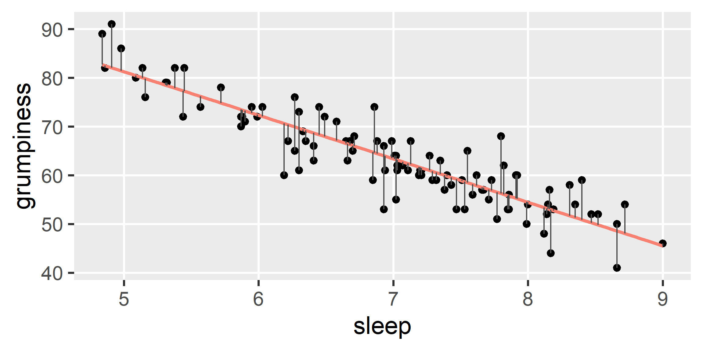
Thus, predictions \((\color{red}{\hat{y}_i})\) differ from the observed values \((y_i)\)
We refer to these differences as the model’s residuals

\[ \begin{align} \color{red}{\hat{y}_i} &= \color{blue}{b_0} + \color{blue}{b_1}x_i\\ y_i &= \color{blue}{b_0} + \color{blue}{b_1}x_i + \color{magenta}{e_i} \\ \color{magenta}{e_i} &= y_i - \color{red}{\hat{y}_i} \end{align} \]

Visualizing Regression Residuals

Minimizing Regression Residuals

If we want the best possible estimates of \(y\), we should…
…look for the line that minimizes the prediction errors
Residuals are the prediction errors
We thus seek to minimize the residuals

But residuals can be positive or negative…
So minimizing the sum of the residuals won’t work
We thus minimize the sum of the squared residuals

OLS Regression

Minimizing the sum of the squared residuals is called OLS
- This stands for “Ordinary Least Squares” Regression
So what are the OLS formulas for the slope and intercept?

\[ b_1 = r_{xy}\frac{s_y}{s_x} \qquad\quad b_0 = \bar{y} - b_1\bar{x} \]

Regression and correlation are thus integrally connected

Example Dataset

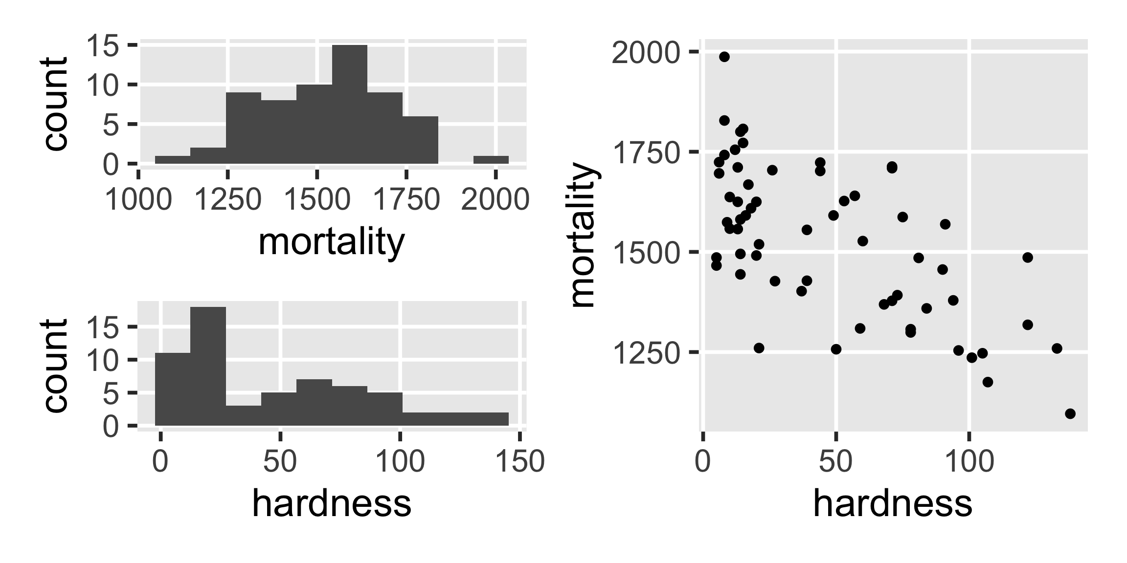
The water dataset has information about mortality and water hardness in 61 UK towns

water <- read_csv("../../data/water.csv")
water

town	location	mortality	hardness
Bath	South	1247	105
Birkenhead	North	1668	17
Birmingham	South	1466	5
Blackburn	North	1800	14
Blackpool	North	1609	18
Bolton	North	1558	10
Bootle	North	1807	15
Bournemouth	South	1299	78
Bradford	North	1637	10
Brighton	South	1359	84
Bristol	South	1392	73
Burnley	North	1755	12
Cardiff	South	1519	21
Coventry	South	1307	78
Croydon	South	1254	96
Darlington	North	1491	20
Derby	North	1555	39
Doncaster	North	1428	39
East Ham	South	1318	122
Exeter	South	1260	21
Gateshead	North	1723	44
Grimsby	North	1379	94
Halifax	North	1742	8
Huddersfield	North	1574	9
Hull	North	1569	91
Ipswich	South	1096	138
Leeds	North	1591	16
Leicester	South	1402	37
Liverpool	North	1772	15
Manchester	North	1828	8
Middlesbrough	North	1704	26
Newcastle	North	1702	44
Newport	South	1581	14
Northampton	South	1309	59
Norwich	South	1259	133
Nottingham	North	1427	27
Oldham	North	1724	6
Oxford	South	1175	107
Plymouth	South	1486	5
Portsmouth	South	1456	90
Preston	North	1696	6
Reading	South	1236	101
Rochdale	North	1711	13
Rotherham	North	1444	14
St Helens	North	1591	49
Salford	North	1987	8
Sheffield	North	1495	14
Southampton	South	1369	68
Southend	South	1257	50
Southport	North	1587	75
South Shields	North	1713	71
Stockport	North	1557	13
Stoke	North	1640	57
Sunderland	North	1709	71
Swansea	South	1625	13
Wallasey	North	1625	20
Walsall	South	1527	60
West Bromwich	South	1627	53
West Ham	South	1486	122
Wolverhampton	South	1485	81
York	North	1378	71

Data Exploration

OLS Regression by Hand

x <- water$hardness
y <- water$mortality

b1 <- cor(x, y) * sd(y) / sd(x)
b1
## [1] -3.226092

b0 <- mean(y) - b1 * mean(x)
b0
## [1] 1676.356

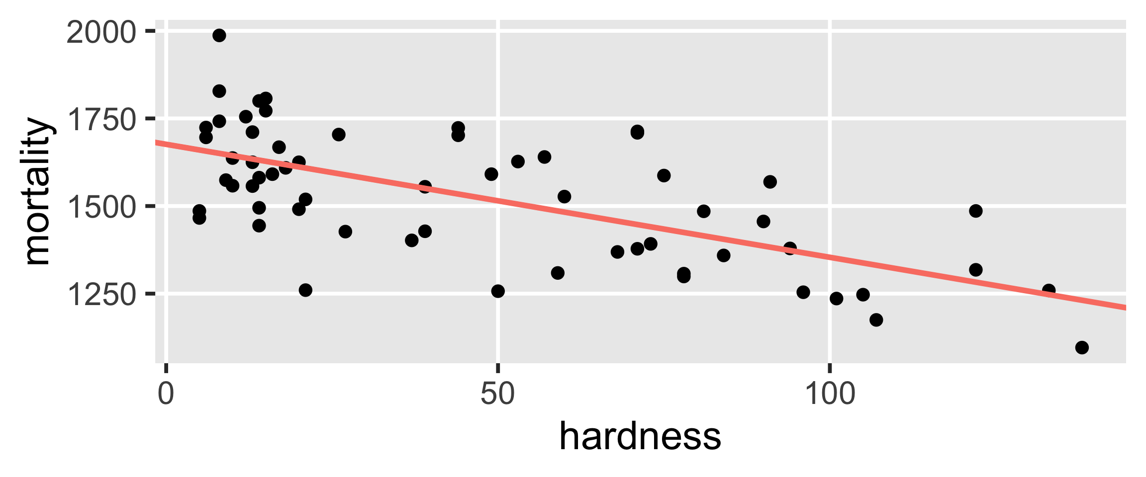
\[ \hat{y}_i = 1676.356 - 3.226 x_i \]

“We estimate that a town with a water hardness of zero would have a mortality of 1676.356. For every one-unit increase in a town’s water hardness, we estimate that its mortality would decrease by 3.226.”

Visualizing our Result

qplot(x = hardness, y = mortality, data = water, geom = "point") + 
  geom_abline(slope = b1, intercept = b0, color = "salmon")

Regression using lm()

fit <- lm(formula = mortality ~ hardness, data = water)
fit
## 
## Call:
## lm(formula = mortality ~ hardness, data = water)
## 
## Coefficients:
## (Intercept)     hardness  
##    1676.356       -3.226

Just like before, the formula is outcome ~ predictor
R refers to \(b_0\) as (Intercept) and \(b_1\) as hardness
This will be helpful when we add multiple predictors

Regression Inference

Uncertainty in the Population

OLS finds the best coefficients for the sample
But we usually care more about the population

Thus, we estimate the population intercept and slope
There will be some inferential uncertainty in this process

As before, we can use NHST and/or estimation approaches
Let’s calculate 95% CIs, test statistics, and \(p\)-values

Slope Confidence Interval

\[ b_1 \pm \text{SE}(b_1)\times t_{crit} \]

\[ \text{SE}(b_1) = \frac{s_y}{s_x}\sqrt{\frac{1-r_{xy}^2}{n-2}} \]

\[t_{crit}\text{ comes from the } t(n-2, 0, 1)\text{ distribution}\]

Intercept Confidence Interval

\[ b_0 \pm \text{SE}(b_0)\times t_{crit} \]

\[ \text{SE}(b_0) = \sqrt{\frac{\sum_i(y_i-\hat{y}_i)^2}{n-2}} \sqrt{\frac{1}{n} + \frac{\bar{x}^2}{(n-1)s_x^2}} \]

\[t_{crit}\text{ comes from the } t(n-2, 0, 1)\text{ distribution}\]

Confidence Intervals in R

fit
## 
## Call:
## lm(formula = mortality ~ hardness, data = water)
## 
## Coefficients:
## (Intercept)     hardness  
##    1676.356       -3.226

confint(fit)
##                  2.5 %      97.5 %
## (Intercept) 1617.73030 1734.980903
## hardness      -4.19602   -2.256163

I’ll show you the {easystats} way after we cover NHST

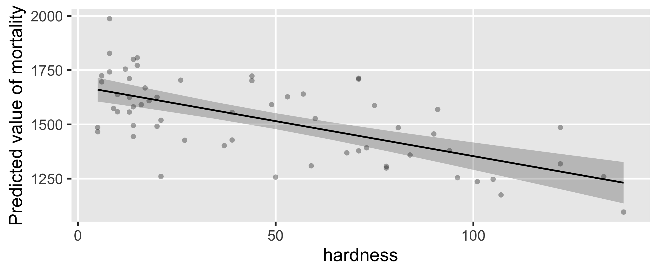
Plotting Regression Results

library(modelbased)
est <- estimate_relation(fit, by = "hardness")
plot(est, show_data = TRUE)

Hypothesis Testing

Null: The true coefficient (in the population) is zero

\[H_0: b = 0\]

Alternative: The true coefficient (in the population) is not zero

\[H_1: b \neq 0\]

Note that this applies to both intercepts and slopes

Testing Individual Coefficients

We can re-use the logic/procedure of the one-sample \(t\)-test
We assume the null sampling distribution for \(\hat{b}\) is normal

\[ t_{obs} = \frac{b}{\text{SE}(b)} \]

\[t_{obs} \sim t(\mathit{df}=n-k-1, \mu=0, \sigma=1)\]

Statistical Inference in R

library(easystats)
model_parameters(fit)
## Parameter   | Coefficient |    SE |             95% CI | t(59) |      p
## -----------------------------------------------------------------------
## (Intercept) |     1676.36 | 29.30 | [1617.73, 1734.98] | 57.22 | < .001
## hardness    |       -3.23 |  0.48 | [  -4.20,   -2.26] | -6.66 | < .001

“A town with zero water hardness is expected to have a mortality rate of 1676.36, which is significantly different from zero, 95% CI: [1617.73, 1734.98], p<.001. For each one-unit increase in water hardness, the model predicts a significant decrease in mortality of 3.23, 95% CI: [–4.20, –2.26], p<.001.”

Centering

Centering a Predictor

The intercept \((b_0)\) is the value of \(\hat{y}\) when \(x=0\)
This isn’t so useful if \(x\) never equals \(0\) in the sample

In such cases, it can be useful to “center” \(x\) before modeling

\[x_i^c = x_i - \bar{x}\]

The slope will stay the same but the intercept will change
The intercept will become the value of \(\hat{y}\) when \(x=\bar{x}\)

Centering a Predictor

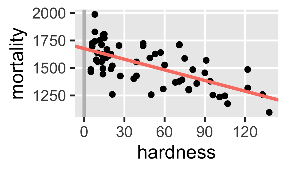
\[b_0 = 1676.356\]

“A town with zero water hardness
would have 1676.356 mortality.”

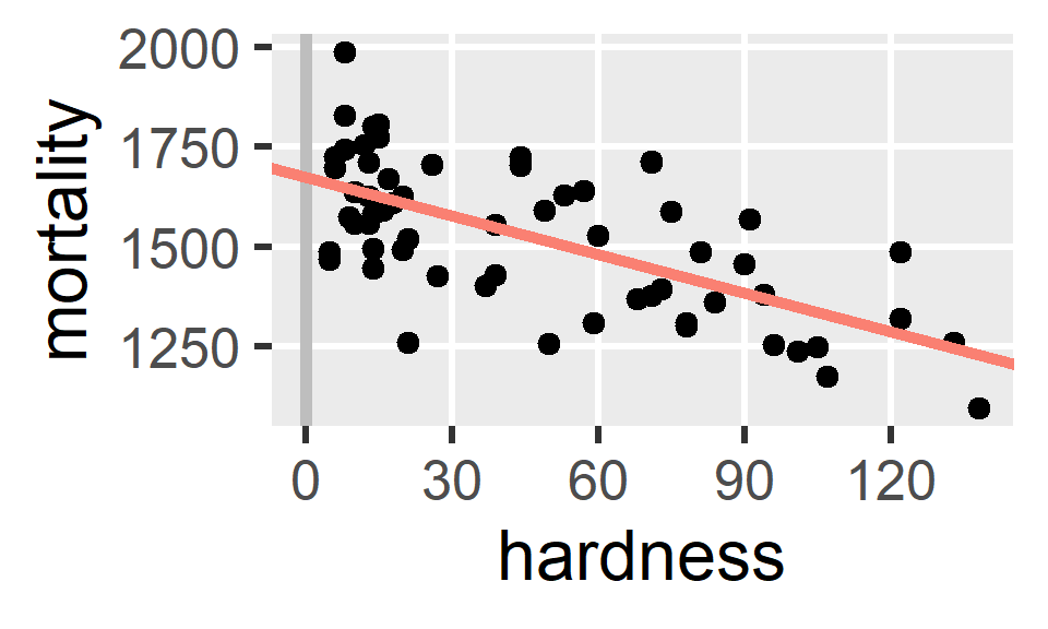
\[b_0 = 1524.148\]

“A town with average water hardness
would have 1524.148 mortality.”

Centering in R

# Two-step process
water$hardness_c <- water$hardness - mean(water$hardness)

fit2a <- lm(formula = mortality ~ hardness_c, data = water)
model_parameters(fit2a)
## Parameter   | Coefficient |    SE |             95% CI | t(59) |      p
## -----------------------------------------------------------------------
## (Intercept) |     1524.15 | 18.31 | [1487.50, 1560.79] | 83.23 | < .001
## hardness c  |       -3.23 |  0.48 | [  -4.20,   -2.26] | -6.66 | < .001

# Or equivalent one-step process
fit2b <- lm(formula = mortality ~ center(hardness), data = water)
model_parameters(fit2b)
## Parameter        | Coefficient |    SE |             95% CI | t(59) |      p
## ----------------------------------------------------------------------------
## (Intercept)      |     1524.15 | 18.31 | [1487.50, 1560.79] | 83.23 | < .001
## center(hardness) |       -3.23 |  0.48 | [  -4.20,   -2.26] | -6.66 | < .001

Regression Effect Sizes

Standardized Slopes

It is common to standardize regression slopes (called \(\beta\)s)
We can do this by standardizing both \(y\) and \(x\) and refitting

\[x_i^z = \frac{x_i - \bar{x}}{s_x} \qquad \quad y_i^z = \frac{y_i - \bar{y}}{s_y}\]

\[\hat{y}_i^z = \beta_0 + \beta_1x_i^z\]

The standardized slope \((\beta_1)\) is interpreted in SD units
The standardized intercept \((\beta_0)\) will equal/approach zero

Standardizing in R

# Method 1: Fit normally then refit
fit <- lm(mortality ~ hardness, data = water)
model_parameters(fit, standardize = "refit")
## Parameter   | Coefficient |   SE |         95% CI |     t(59) |      p
## ----------------------------------------------------------------------
## (Intercept) |   -4.55e-16 | 0.10 | [-0.20,  0.20] | -4.66e-15 | > .999
## hardness    |       -0.65 | 0.10 | [-0.85, -0.46] |     -6.66 | < .001

# Method 2: Standardize data then fit
fit2 <- lm(mortality ~ hardness, data = standardize(water))
model_parameters(fit2)
## Parameter   | Coefficient |   SE |         95% CI |     t(59) |      p
## ----------------------------------------------------------------------
## (Intercept) |   -4.55e-16 | 0.10 | [-0.20,  0.20] | -4.66e-15 | > .999
## hardness    |       -0.65 | 0.10 | [-0.85, -0.46] |     -6.66 | < .001

“For each one SD increase in water hardness, we would expect a 0.65 SD
decrease in mortality, \(\beta=-0.65\), 95% CI: \([-0.85, -0.46]\), \(p<.001\).”

R-Squared

\(R^2\) is the variance in \(y\) explained by the regression model
- Ranges from 0.0 (0% explained) to 1.0 (100% explained)
- It is equivalent to squaring the correlation of \(y\) and \(\hat{y}\)
- It is also called the “coefficient of determination”

\[ R^2 = 1 - \frac{\text{SS}_{res}}{\text{SS}_{tot}} = 1 - \frac{\sum_i(y_i - \hat{y}_i)^2}{\sum_i(y_i - \bar{y})^2} \]

Adjusted R-Squared

\(R^2\) will never decrease when adding more predictors
So we often adjust it to penalize adding more predictors

\[ R_{adj}^2 = 1 - \left(\frac{\text{SS}_{res}}{\text{SS}_{tot}} \times \frac{n - 1}{n - k - 1}\right) \]

Negative values of \(R_{adj}^2\) are possible
Its interpretation is less straightforward

Model Performance in R

# By hand (with the residuals function shortcut)
R2a <- 1 - sum(residuals(fit)^2) / sum((y - mean(y))^2)
R2a
## [1] 0.4288267

# By function (recommended)
R2b <- r2(fit, ci = 0.95)
R2b
##        R2: 0.429 [0.230, 0.601]
##   adj. R2: 0.419 [0.220, 0.593]

“The regression model in which mortality was regressed on water hardness explained 42.9% of the variance in mortality, R² = 0.429, 95% CI: [0.230, 0.601], Adjusted R² = 0.419.”