Statistical Methods with R

ANOVA Extensions

Unit B · Chapter 06 · Lecture 06c

Developed by Jeffrey M. Girard

Unequal Variances

Welch’s one-way test

The ANOVA we learned in the previous lecture used Student’s approach
- It simplifies the math by assuming all \(\sigma\) are equal
- The “homogeneity of variance” or “sphericity” assumption
But we can extend Welch’s approach to ANOVA as well
- This will let us relax this assumption
- The math is more complex than we have time for
- But I will show you how to implement it

Example dataset

library(tidyverse)
penguins <- read_csv("../../data/penguins.csv")
penguins
## # A tibble: 344 × 8
##    species island    bill_len bill_dep flipper_len body_mass sex     year
##    <chr>   <chr>        <dbl>    <dbl>       <dbl>     <dbl> <chr>  <dbl>
##  1 Adelie  Torgersen     39.1     18.7         181      3750 male    2007
##  2 Adelie  Torgersen     39.5     17.4         186      3800 female  2007
##  3 Adelie  Torgersen     40.3     18           195      3250 female  2007
##  4 Adelie  Torgersen     NA       NA            NA        NA <NA>    2007
##  5 Adelie  Torgersen     36.7     19.3         193      3450 female  2007
##  6 Adelie  Torgersen     39.3     20.6         190      3650 male    2007
##  7 Adelie  Torgersen     38.9     17.8         181      3625 female  2007
##  8 Adelie  Torgersen     39.2     19.6         195      4675 male    2007
##  9 Adelie  Torgersen     34.1     18.1         193      3475 <NA>    2007
## 10 Adelie  Torgersen     42       20.2         190      4250 <NA>    2007
## # ℹ 334 more rows

Exploratory analysis

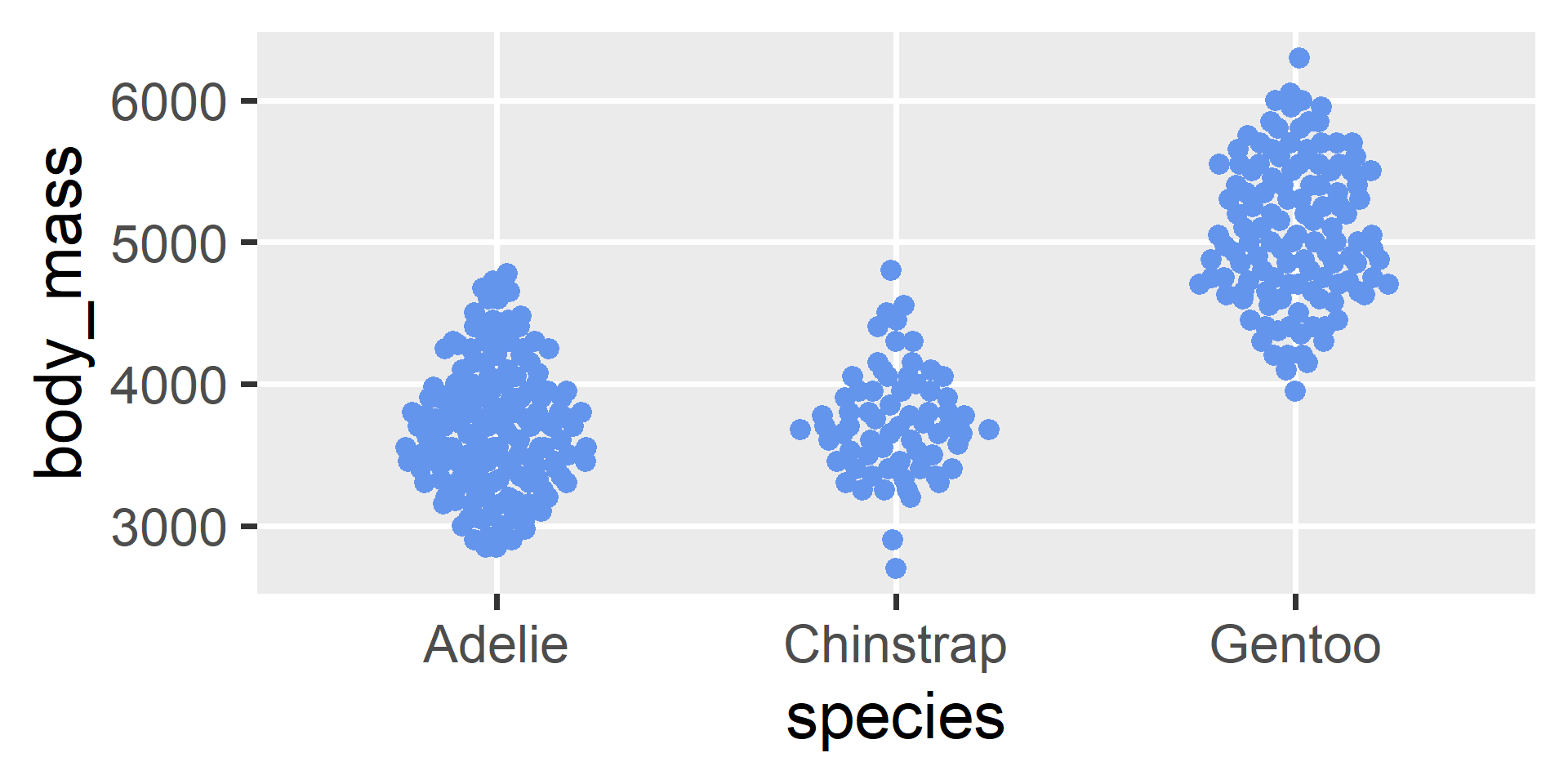
Welch’s test in R

library(easystats)

fit <- oneway.test(
  formula = body_mass ~ species,
  data = penguins
)

model_parameters(fit)
## One-way analysis of means (not assuming equal variances)
## 
## F      | df | df (error) |      p
## ---------------------------------
## 317.57 |  2 |     189.48 | < .001

Repeated Measures

One-way RM ANOVA

To compare independent groups, we can use…
- Independent samples \(t\)-test (for exactly 2 groups)
- One-way ANOVA (for 3+ groups)
To compare dependent/paired groups, we can use…
- Paired samples \(t\)-test
- One-way Repeated Measures ANOVA

Further partitioning

We will partition the variation into three final components

%%{ init: {
    "theme": "base",
    "themeVariables": { "fontSize": "24px" }
} }%%

flowchart LR
  T[Total Variation] --> B(Between-Group Variation)
  T --> W(Within-Group Variation)
  W --> S(Subject Variation)
  W --> E(Error Variation)

Independent Samples \[F_{obs} = \frac{MS_b}{MS_w}\]

Dependent Samples \[F_{obs} = \frac{MS_b}{MS_e}\]

Partitioning the variation

\[\text{SS}_b = \sum_{k=1}^g n_k(\bar{y}_k - \bar{y})^2 \qquad \text{SS}_w = \sum_{k=1}^g\sum_{i=1}^{n_k}(y_{ik} - \bar{y}_k)^2\]

How far are group means from the grand mean?

How far are scores from their group means?

\[\quad \color{red}{\text{SS}_s = g \sum_{i=1}^{n} (\bar{y}_i - \bar{y})^2 \qquad \quad \text{SS}_e = \text{SS}_w - \text{SS}_s} \qquad \qquad\]

How far are subject means from the grand mean?

How much variation is not yet explained?

The One-way RM ANOVA

Mean Squares and Degrees of Freedom

\[\text{MS}_b = \frac{\text{SS}_b}{g - 1} \qquad \text{MS}_e = \frac{\text{SS}_e}{(n-1)(g-1)}\]

Test Statistic and Null Sampling Distribution

\[ F_{obs} = \frac{\text{MS}_b}{\text{MS}_e} \\ F_{obs} \sim F(\textit{df}_1=g-1, \textit{df}_2 = (n-1)(g-1)) \]

Example data

depression <- read_csv("../../data/depression.csv")
depression
## # A tibble: 162 × 3
##    patient time   hrsd
##      <dbl> <chr> <dbl>
##  1       1 t0       19
##  2       1 t1        8
##  3       1 t2       13
##  4       2 t0       20
##  5       2 t1       21
##  6       2 t2       13
##  7       3 t0       14
##  8       3 t1        7
##  9       3 t2        8
## 10       4 t0       16
## # ℹ 152 more rows

Exploratory analysis

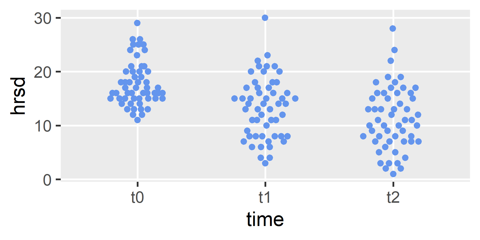
Fitting the model in R

library(afex)
fit <- aov_4(
  formula = hrsd ~ (time | patient),
  data = depression
)
model_parameters(fit)
## ANOVA estimation for factorial designs using 'afex'
## 
## Parameter | Sum_Squares | Sum_Squares_Error |   df | df (error) | Mean_Square
## -----------------------------------------------------------------------------
## time      |     1166.26 |           1231.07 | 1.86 |      98.64 |       12.48
## 
## Parameter |     F |      p
## --------------------------
## time      | 50.21 | < .001
## 
## Anova Table (Type 3 tests)

Estimating means

gmeans <- estimate_means(fit, by = "time")
gmeans
## Estimated Marginal Means
## 
## time |  Mean |   SE |         95% CI | t(53)
## --------------------------------------------
## t0   | 17.76 | 0.57 | [16.62, 18.89] | 31.39
## t1   | 13.35 | 0.77 | [11.81, 14.89] | 17.37
## t2   | 11.33 | 0.80 | [ 9.73, 12.93] | 14.22
## 
## Variable predicted: hrsd
## Predictors modulated: time
## Predictors averaged: patient

Plotting means

plot(gmeans)

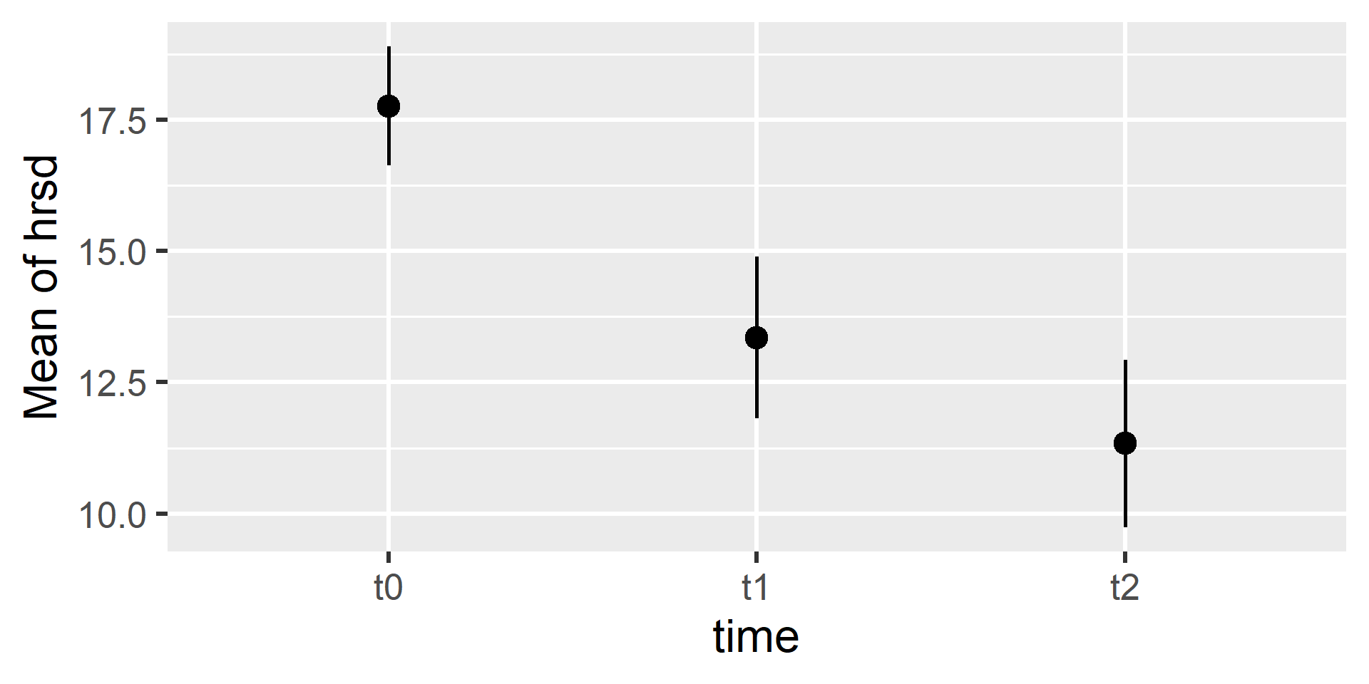
The partial eta-squared effect size

How much of the non-subject variation is between groups?

\[\eta_{partial}^2 = \frac{\text{SS}_b}{\text{SS}_b + \text{SS}_e}\]

eta_squared(fit)
## # Effect Size for ANOVA (Type III)
## 
## Parameter | Eta2 (partial) |       95% CI
## -----------------------------------------
## time      |           0.49 | [0.37, 1.00]
## 
## - One-sided CIs: upper bound fixed at [1.00].

Post-hoc tests

We can average pairwise time-contrasts over patients
e.g., what is the T1–T0 difference for the average patient?

estimate_contrasts(
  model = fit,
  contrast = "time",
  method = "pairwise"
)
## Marginal Contrasts Analysis
## 
## Level1 | Level2 | Difference |   SE |         95% CI | t(53) |      p
## ---------------------------------------------------------------------
## t1     | t0     |      -4.41 | 0.70 | [-5.81, -3.01] | -6.32 | < .001
## t2     | t0     |      -6.43 | 0.70 | [-7.83, -5.02] | -9.17 | < .001
## t2     | t1     |      -2.02 | 0.56 | [-3.14, -0.90] | -3.61 | < .001
## 
## Variable predicted: hrsd
## Predictors contrasted: time
## Predictors averaged: patient
## p-values are uncorrected.

Translation Activity

Example 1 (Social Psych)

I read about a theory that says that a common enemy can unite political rivals. To test this, I have 200 American participants first complete a measure of hostility toward members of the opposing political party. They then read a news article that describes a foreign government threatening the USA. After answering some basic questions about the article, the participants complete another measure of hostility toward members of the opposing political party. Both measures of hostility are continuous and range from \(-5\) to \(5\).

What might the data frame look like for this study?
What might my null and alternative hypotheses be?
What statistical test(s) from this course might I use here?

Example 2 (Clinical Psych)

I read about a theory that says that the personality trait of “Openness to Experience” (from the Big 5) is related to psychosis such that people with higher levels of this personality trait experience more symptoms of psychosis (e.g., hallucinations, delusions, and disorganized thinking) on average. To explore this idea, I collect data from 150 members of my local community, including self-report measures of the Big 5 personality traits and psychotic symptoms. All these measures are continuous and range from \(0\) to \(100\).

What might the data frame look like for this study?
What might my null and alternative hypotheses be?
What statistical test(s) from this course might I use here?

Example 3 (Sports Science)

I read about a new pre-workout stretching technique that is supposed to dramatically reduce cramping. To see if it really works, I instruct one-third of the players on the soccer team I coach to use the new technique at the start of practice, another third to use a traditional stretching technique, and the final third to not stretch at all. After practice, I collect reports from each player on how much cramping they experienced during practice (on a scale from \(1\) to \(10\)).

What might the data frame look like for this study?
What might my null and alternative hypotheses be?
What statistical test(s) from this course might I use here?

Small-Group Activity

Step 1. Write down a few of your own examples (e.g., 2 to 4). The hypotheses should be testable using one-sample \(t\)-tests, two-sample \(t\)-tests, one-way tests, or correlations.

Step 2. Form small groups of two to three students and take turns reading each others’ examples. Discuss the answers to our three questions and brainstorm together.

What might the data frame look like for this study?
What might my null and alternative hypotheses be?
What statistical test(s) from this course might I use here?