library(tidyverse)
penguins <- read_csv("penguins.csv")
penguins
## # A tibble: 344 × 8
##    species island    bill_len bill_dep flipper_len body_mass sex     year
##    <chr>   <chr>        <dbl>    <dbl>       <dbl>     <dbl> <chr>  <dbl>
##  1 Adelie  Torgersen     39.1     18.7         181      3750 male    2007
##  2 Adelie  Torgersen     39.5     17.4         186      3800 female  2007
##  3 Adelie  Torgersen     40.3     18           195      3250 female  2007
##  4 Adelie  Torgersen     NA       NA            NA        NA <NA>    2007
##  5 Adelie  Torgersen     36.7     19.3         193      3450 female  2007
##  6 Adelie  Torgersen     39.3     20.6         190      3650 male    2007
##  7 Adelie  Torgersen     38.9     17.8         181      3625 female  2007
##  8 Adelie  Torgersen     39.2     19.6         195      4675 male    2007
##  9 Adelie  Torgersen     34.1     18.1         193      3475 <NA>    2007
## 10 Adelie  Torgersen     42       20.2         190      4250 <NA>    2007
## # ℹ 334 more rowsStatistical Methods with R
Comparing Many Groups
Unit B · Chapter 06 · Lecture 06b
Developed by Jeffrey M. Girard

Roadmap: Group Comparisons
Introduction
One-way ANOVA in R
Post-hoc Tests
Introduction
Rationale
The t-test compares two groups’ population means
But sometimes we want to compare three or more groups
This is what one-way analysis of variance (ANOVA) does
- One-way focuses on one source of variance (i.e., groups)
- The one-way ANOVA is for independent samples/groups
H_0: \text{it is true that } \mu_1=\mu_2=\mu_3 \cdots \\ H_1: \text{it is NOT true that } \mu_1=\mu_2=\mu_3 \cdots
Example dataset
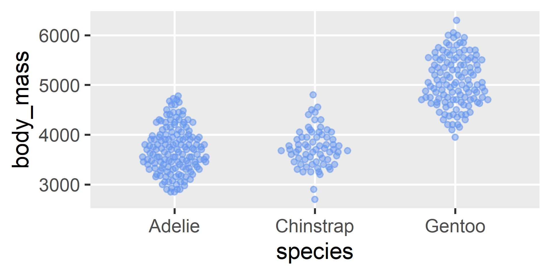
- Do the three penguin species have the same mean body mass?
Exploratory analysis
Total variance
Across all observations (in all groups), what is the average squared difference between each observation and the global mean (calculated across all observations in all groups)?
\text{Var}(y)=\frac{1}{n}\sum_{i=1}^n(y_i - \bar{y})^2
n is the total sample size across all groups
\bar{y} is the global mean of y across all groups
Sums of squares
- ANOVA uses sums of squares (SS) rather than variances
- SS are the same as variances but don’t divide by n
- They are the sums of squared differences (not the means)
\color{blue}{\text{SS}_{tot}=\sum_{i=1}^n(y_{i}-\bar{y})^2}
\text{Var}(y)=\frac{1}{n}\sum_{i=1}^n(y_{i} - \bar{y})^2
Using SS yields a nicer interpretation and enables the use of the F distribution
Between and within groups
- The total variation (SS_{tot}) contains two components
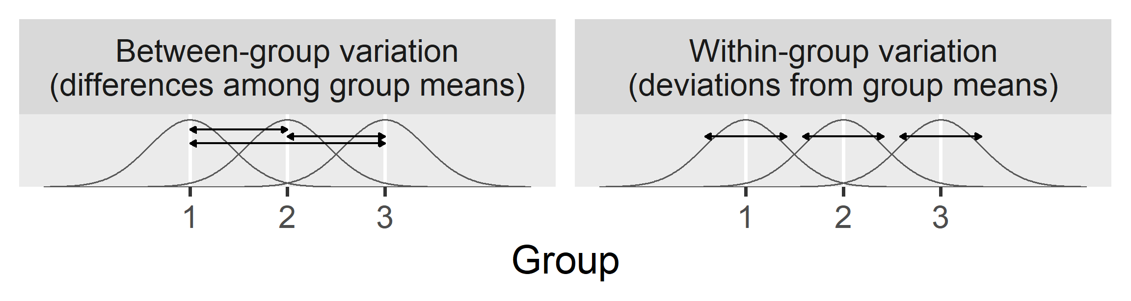
How different are the three groups/species (on average)?
How different are penguins
in the same group/species?
Decomposing the variation
- We can decompose total variation into two components:
Between-group variation
\text{SS}_b = \sum_{k=1}^gn_k(\bar{y}_k - \bar{y})^2
How far is each group mean \bar{y}_k from the global mean \bar{y}?
Within-group variation
\text{SS}_w = \sum_{k=1}^g\sum_{i=1}^{n_k}(y_{ik} - \bar{y}_k)^2
How far is each observation y_{ik} from its group mean \bar{y}_k?
Note that the decomposition ensures that SS_{tot}=SS_b + SS_w
Testing for mean differences
- If H_0 is true, the groups’ population means are the same
- Thus, between-group variation (SS_b) should be small
- But how small is small enough? We need to contextualize it
- ANOVA does so by comparing SS_b to SS_w
- It focuses on the ratio of SS_b to SS_w (i.e., SS_b/SS_w)
- But we need to build in the group and sample sizes
- Doing so will allow us to calibrate our uncertainty
Incorporating uncertainty
Mean Squares Between
\textit{MS}_b = \frac{\textit{SS}_b}{g - 1}
Mean Squares Within
\textit{MS}_w = \frac{\textit{SS}_w}{n - g}
The One-way ANOVA Test Statistic F_{obs} = \frac{\textit{MS}_b}{\textit{MS}_w}\\ F_{obs} \sim F(\textit{df}_1 = g - 1, \textit{df}_2 = n - g)
g is the number of groups, n is the total sample size
The F distribution
The sum of squared standard normals has a \chi^2 distribution
The ratio of two independent \chi^2 variables, each divided by its df, is F-distributed
This is why F uses MS = SS/\textit{df}
x \sim F(\textit{df}_1, \textit{df}_2)
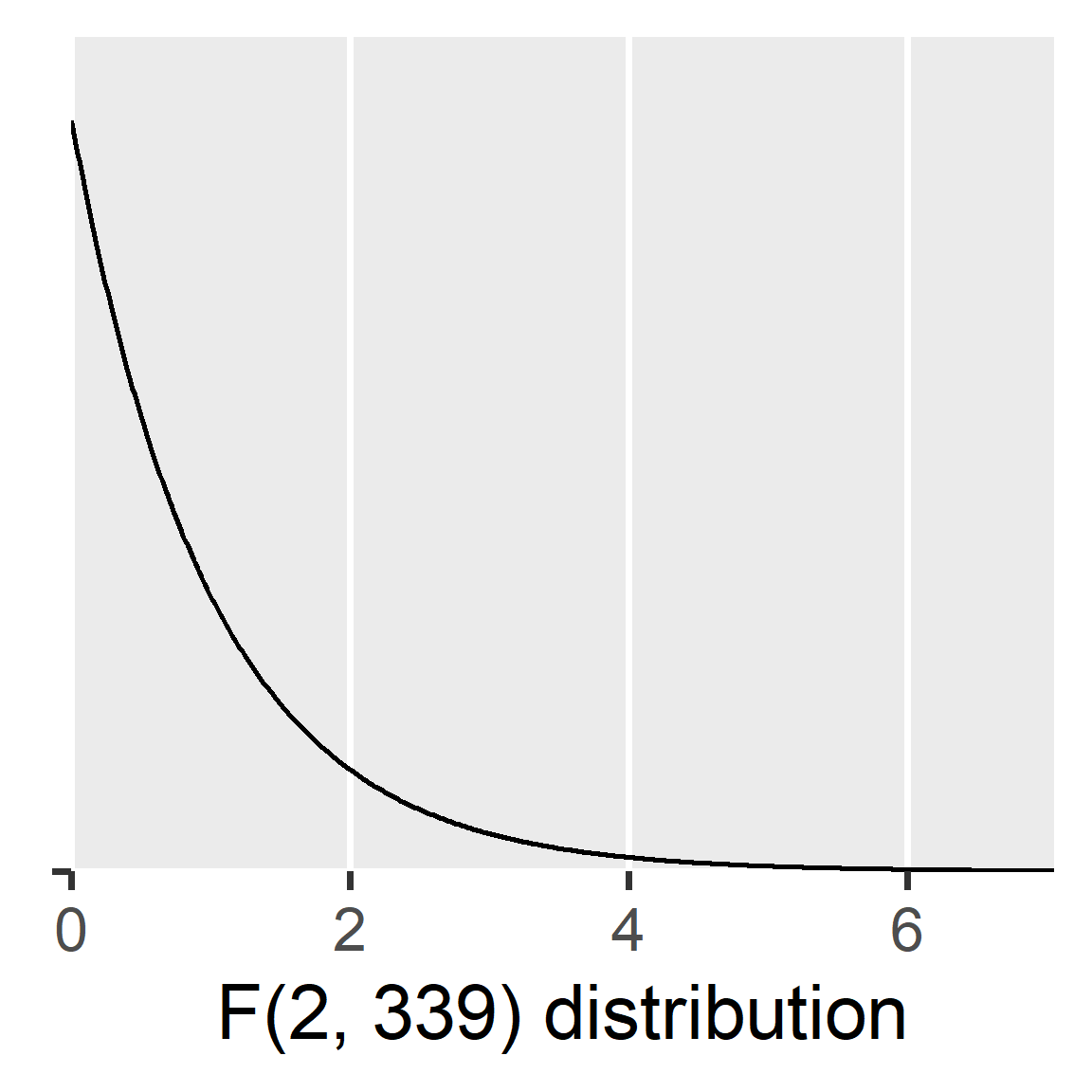
The df1 parameter
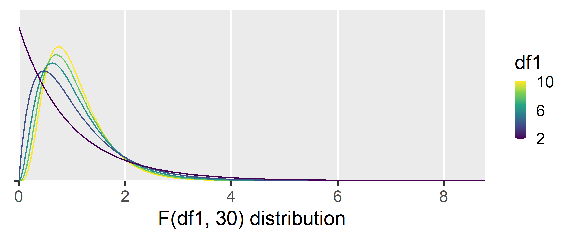
- Higher \textit{df}_1 has thinner tails (i.e., lower critical values)
The df2 parameter
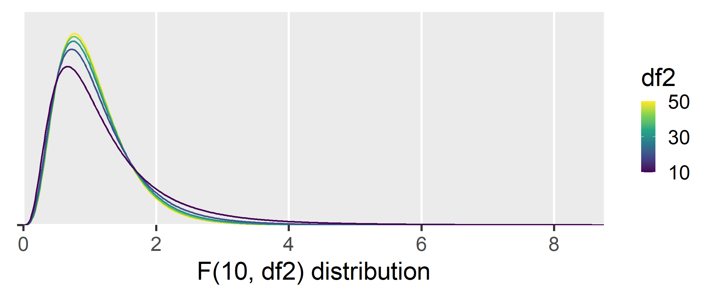
- Higher \textit{df}_2 has thinner tails (i.e., lower critical values)
One-way ANOVA in R
The aov function
- The
aov()function will do this math for us
Prettier output
We used a one-way ANOVA to compare the mean body masses of Adelie, Chinstrap, and Gentoo penguins and rejected the null hypothesis that these three groups have the same mean, F(2,339)=343.63, p<.001.
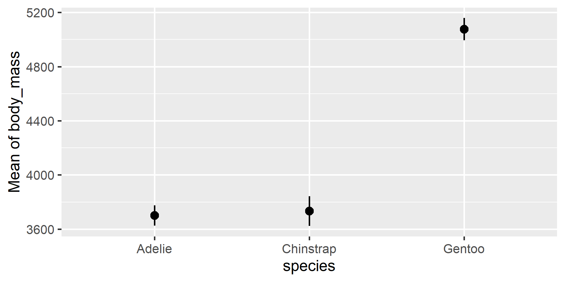
Estimating group means
- We can also estimate the model-implied group means
gmeans <- estimate_means(fit, by = "species")
gmeans
## Estimated Marginal Means
##
## species   |    Mean |    SE |             95% CI | t(339)
## ---------------------------------------------------------
## Adelie    | 3700.66 | 37.62 | [3626.67, 3774.66] |  98.37
## Chinstrap | 3733.09 | 56.06 | [3622.82, 3843.36] |  66.59
## Gentoo    | 5076.02 | 41.68 | [4994.03, 5158.00] | 121.78
##
## Variable predicted: body_mass
## Predictors modulated: species
Note that this function requires the {emmeans} package to be installed
Plotting group means
An effect size for One-way ANOVA
We conclude that H_0 is wrong, but how wrong was it?
How much of the total variation was between groups?
\eta^2 = \frac{SS_b}{SS_{tot}}
If \eta^2=0, then none of the variation was between groups
If \eta^2=1, then all of the variation was between groups
Application and interpretation
- So 67% of the variation in body mass was between groups/species
Post-hoc Tests
Many ways to reject the null
- Recall that our null hypothesis is that \mu_1=\mu_2=\mu_3
| Possibility | \mu_1=\mu_2 | \mu_1=\mu_3 | \mu_2=\mu_3 | Hypothesis |
|---|---|---|---|---|
| 1 | TRUE | TRUE | TRUE | null |
| 2 | TRUE | - | - | alternative |
| 3 | - | TRUE | - | alternative |
| 4 | - | - | TRUE | alternative |
| 5 | - | - | - | alternative |
Equality is transitive, so no other combinations are possible: if \mu_1=\mu_3 and \mu_2=\mu_3, then \mu_1=\mu_2
- Thus, if we reject the null, we don’t know exactly why…
Pairwise t-tests
- To figure it out, we can run a t-test for each pair of groups
- These are called “post hoc” (Latin for “after that”) tests
\mu_1=\mu_2 \qquad \mu_1=\mu_3 \qquad \mu_2=\mu_3
- There are two main challenges with this approach
- It will be a hassle to run all these tests as g increases
- Running many tests will increase the Type I Error rate
Addressing the challenges
- For the first challenge, we will use programming
- We will use R functions to do all the work for us
- For the second challenge, we will use two approaches
- Gating: only run post-hoc tests if ANOVA is significant
- p-value adjustment: increase p based on # of tests run
- We want to keep the overall (“familywise”) error rate at \alpha
- We will learn two common adjustment approaches
Gating is a common convention (adjustment alone also controls the familywise rate); we will follow it in this course
Bonferroni correction
- Multiply each p by the number of tests run (m)
p' = p \times m
| raw p | m | Bonferroni p' |
|---|---|---|
| .001 *** | 5 | .005 ** |
| .005 ** | 5 | .025 * |
| .019 * | 5 | .095 |
| .022 * | 5 | .110 |
| .103 | 5 | .515 |
Bonferroni is simple but very conservative
Holm correction
Pretend you do the tests from smallest to largest p-value
Take the larger of (p'_j=j\times p_j) and (p'_{j+1})
| raw p | rank j | p\times j | Holm p' |
|---|---|---|---|
| .001 *** | 5 | .005 | .005 ** |
| .005 ** | 4 | .020 | .020 * |
| .019 * | 3 | .057 | .057 |
| .022 * | 2 | .044 | .057 |
| .103 | 1 | .103 | .103 |
Holm is complicated but more powerful
Post-hoc tests in R
estimate_contrasts(
  model = fit,
  contrast = "species",
  method = "pairwise",
  p_adjust = "bonferroni"
)
## Marginal Contrasts Analysis
##
## Level1    | Level2    | Difference |    SE |             95% CI | t(339) |      p
## ---------------------------------------------------------------------------------
## Chinstrap | Adelie    |      32.43 | 67.51 | [-100.37,  165.22] |   0.48 | > .999
## Gentoo    | Adelie    |    1375.35 | 56.15 | [1264.91, 1485.80] |  24.50 | < .001
## Gentoo    | Chinstrap |    1342.93 | 69.86 | [1205.52, 1480.34] |  19.22 | < .001
##
## Variable predicted: body_mass
## Predictors contrasted: species
## p-value adjustment method: Bonferroni
Adjustment in R
estimate_contrasts(
  model = fit,
  contrast = "species",
  method = "pairwise",
  p_adjust = "holm" # change the method here
)
## Marginal Contrasts Analysis
##
## Level1    | Level2    | Difference |    SE |             95% CI | t(339) |      p
## ---------------------------------------------------------------------------------
## Chinstrap | Adelie    |      32.43 | 67.51 | [-100.37,  165.22] |   0.48 |  0.631
## Gentoo    | Adelie    |    1375.35 | 56.15 | [1264.91, 1485.80] |  24.50 | < .001
## Gentoo    | Chinstrap |    1342.93 | 69.86 | [1205.52, 1480.34] |  19.22 | < .001
##
## Variable predicted: body_mass
## Predictors contrasted: species
## p-value adjustment method: Holm (1979)