library(tidyverse)
tratings <- read_csv("teaching_ratings.csv")
tratings
## # A tibble: 94 × 9
##     prof   age sex    minority native track beauty  eval courses
##    <dbl> <dbl> <chr>     <dbl>  <dbl> <dbl>  <dbl> <dbl>   <dbl>
##  1     1    36 female        1      1     1   0.29  4          4
##  2     2    59 male          0      1     1  -0.74  3.53       3
##  3     3    51 male          0      1     1  -0.57  3.45       2
##  4     4    40 female        0      1     1  -0.68  4.01       8
##  5     5    31 female        0      1     1   1.51  4.35       6
##  6     6    62 male          0      1     1   0.59  4.44       7
##  7     7    33 female        0      1     1  -0.13  3.84       5
##  8     8    51 female        0      1     1  -0.26  4.03       7
##  9     9    33 female        0      1     1   0.15  4.26       7
## 10    10    47 male          0      1     2   0.54  4.56      10
## # ℹ 84 more rowsStatistical Methods with R
Comparing Two Groups
Unit B · Chapter 06 · Lecture 06a
Developed by Jeffrey M. Girard

Roadmap: Group Comparisons
Introductions
NHST Approaches
Effect Sizes
Introductions
Group Comparisons
Many research questions are about comparing groups
Do two (or more) groups have the same population mean?
- These groups may be naturally occurring
(e.g., Do adults or children watch more TV?) - Or they may correspond to experimental conditions
(e.g., Do outcomes differ in treatment and placebo?) - Two groups of measurements may be related/paired
(e.g., Is a person’s memory better before or after exercise?)
- These groups may be naturally occurring
Types of Groups
We will collect a sample of data from each group
Independent Samples: Observations are unrelated
- e.g., Each participant only occurs in a single group/sample
- e.g., Different people are assigned to condition A or B
Dependent/Paired Samples: Observations are linked
- e.g., Each participant occurs in multiple groups/samples
- e.g., Each person participates in both condition A and B
Types of Comparisons
Significance Testing
Is the difference between the two group means zero?
The result is a test statistic,
p-value, and decision to retain or reject the nullAdults watch significantly more TV than do children, t(99)=20.14, p<.001
Estimation
What are reasonable values for the difference between the two group means?
The result is a point estimate and interval estimate (CI)
Adults watch 3.2 more hours of TV per day than do children, 95% CI: [1.8, 4.6]
NHST Approaches
Recap of Steps in NHST
Set null and alternative hypotheses, Type I Error Rate (\alpha)
Choose an appropriate test and calculate its test statistic
Estimate null sampling distribution for test statistic
Calculate critical values from null sampling distribution
Compare the observed test statistic to these critical values
Calculate \boldsymbol{p}-value and decide to retain or reject the null
Independent Samples t-test
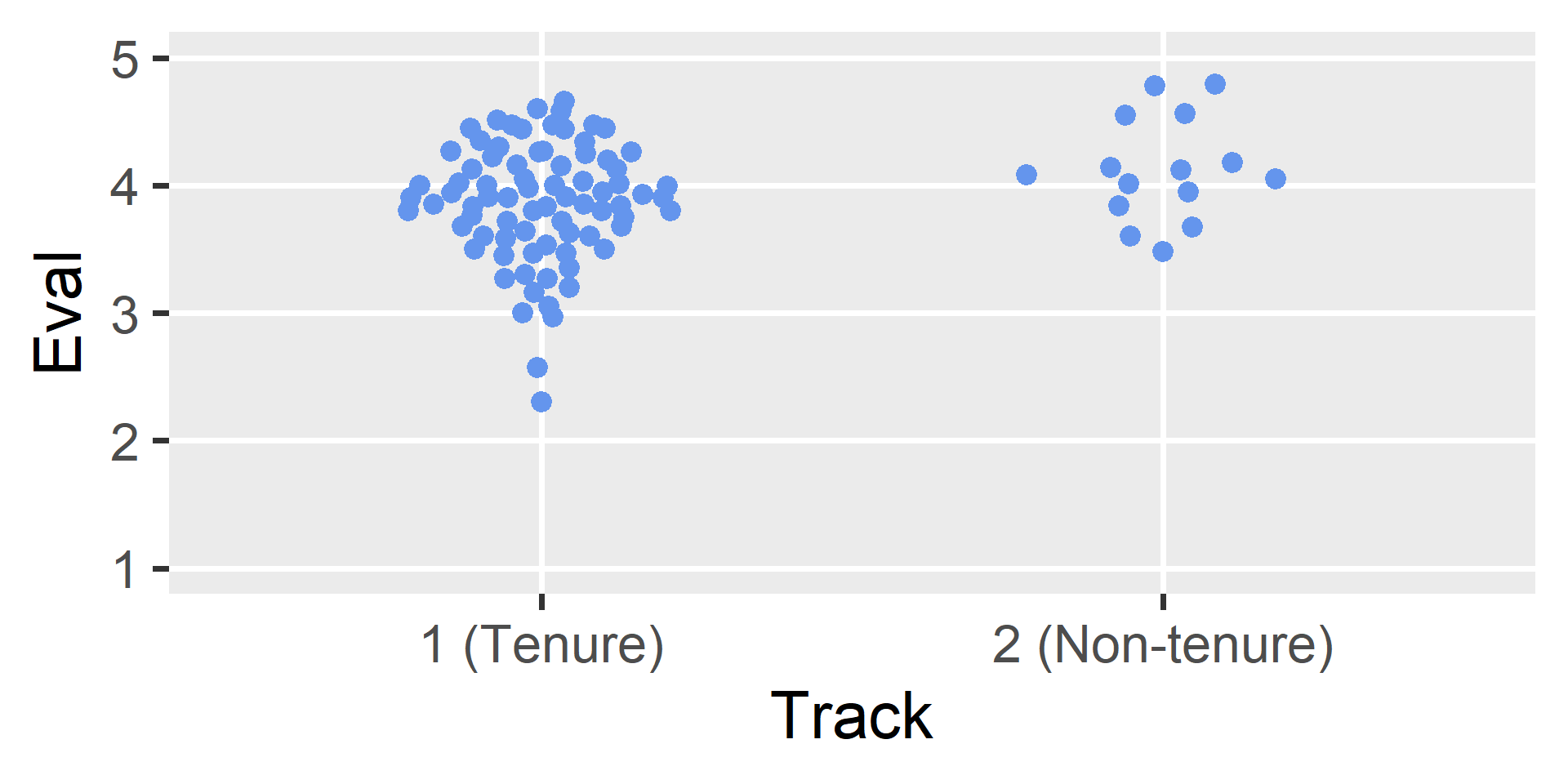
Research Question: Do tenure track (G1) or non-tenure track (G2) professors receive better teaching evals, on average?
Each professor is G1 or G2, so these are independent groups
- Are the G1 and G2 samples drawn from populations with
the same mean (null) or different means (alternative)?
H_0: \mu_1=\mu_2\\ H_1: \mu_1\neq\mu_2
Example data
Data Exploration
Test Statistic
If the null is true and \mu_1 = \mu_2, then \mu_1 - \mu_2 = 0
We can use this as the basis of our test statistic
But again, the math is easier if we standardize it
t_{diff}=\frac{\bar{x}_1 - \bar{x}_2}{SE_{diff}}
- So now we just need to estimate the SE of the difference
Two approaches
There are two main approaches to estimating SE_{diff}
Student’s approach assumes “equal variance”
- It assumes that both populations have the same SD
- In parameter terms, it assumes that \sigma_1 = \sigma_2
- This approach simplifies the math, so we start here
Welch’s approach does not make this assumption
- It has a more complicated equation
- But it is usually more realistic
Student’s approach
- We can estimate \sigma by “pooling” s_1 and s_2
s_p = \sqrt{\frac{s_1^2(n_1-1) + s_2^2(n_2-1)}{n_1+n_2-2}}
- We can now use s_p to estimate SE_{diff}
SE_{diff} = s_p \sqrt{\frac{1}{n_1} + \frac{1}{n_2}}
Pooling is taking a weighted average (weighted by sample size minus 1).
Student’s approach
- Our test statistic for Student’s approach is:
t_{diff} = \frac{\bar{x}_1 - \bar{x}_2}{s_p\sqrt{\frac{1}{n_1} + \frac{1}{n_2}}}
- The null sampling distribution is assumed to be:
t_{diff} \sim t(\textit{df}=n_1+n_2-2, \mu=0, \sigma=1)
Welch’s approach
SE_{diff} = \sqrt{\frac{s_1^2}{n_1} + \frac{s_2^2}{n_2}}
t_{diff} \sim t\left( \textit{df}=\frac{\left(\frac{s_1^2}{n_1} + \frac{s_2^2}{n_2}\right)^2} {\frac{\left(\frac{s_1^2}{n_1}\right)^2}{n_1-1} + \frac{\left(\frac{s_2^2}{n_2}\right)^2}{n_2-1}}, \mu=0, \sigma=1\right)
Both approaches in R
- We can have R do all this math for us using
t.test()formula: in the format outcome ~ groupdata: tibble containing outcome and groupvar.equal: TRUE (Student’s) or FALSE (Welch’s)
Student’s test results
fit_s <- t.test(
formula = eval ~ track,
data = tratings,
var.equal = TRUE
)
library(easystats)
model_parameters(fit_s)
## Two Sample t-test
##
## Parameter | Group | track = 1 | track = 2 | Difference | 95% CI | t(92) | p
## ---------------------------------------------------------------------------------------
## eval | track | 3.87 | 4.12 | -0.25 | [-0.51, 0.00] | -1.99 | 0.049
##
## Alternative hypothesis: true difference in means between group 1 and group 2 is not equal to 0- 1
-
Be sure to set
var.equal=TRUEto use Student’s approach
“A Student’s independent samples t-test found that tenure-track professors’ average eval (M=3.87) was significantly lower than non-tenure-track professors’ average eval (M=4.12), t(92)=–1.99, p=.049. The difference was estimated to be –0.25, 95% CI: [–0.51, 0.00].”
Note that this result is barely significant.
Welch’s approach in R
fit_w <- t.test(
formula = eval ~ track,
data = tratings,
var.equal = FALSE
)
model_parameters(fit_w)
## Welch Two Sample t-test
##
## Parameter | Group | track = 1 | track = 2 | Difference | 95% CI
## -----------------------------------------------------------------------
## eval | track | 3.87 | 4.12 | -0.25 | [-0.50, -0.01]
##
## Parameter | t(21.62) | p
## ----------------------------
## eval | -2.19 | 0.040
##
## Alternative hypothesis: true difference in means between group 1 and group 2 is not equal to 0- 1
-
Be sure to set
var.equal=FALSEto use Welch’s approach
“A Welch’s independent samples t-test found that tenure-track professors’ average eval (M=3.87) was significantly lower than non-tenure-track professors’ average eval (M=4.12), t(21.62)=–2.19, p=.040. The difference was estimated to be –0.25, 95% CI: [–0.50, –0.01].”
Paired groups
- Sometimes observations in our groups are related
- Observation X in G1 is related somehow to observation X in G2
- e.g., repeated measures of the same person or thing
- If we ignore these relationships in our modeling…
- Our SE estimates will tend to be too high (when the pairing correlation is positive)
- So our p-values and CIs are wrong, costing power
Paired samples t-test
- To fix this, we can calculate the paired differences
\Delta_i = x_{1i} - x_{2i}
- Then we do a one-sample t-test on the differences
t_\Delta = \frac{\bar{\Delta}}{SE_{\bar{\Delta}}} = \frac{\bar{\Delta}}{s_{\Delta}/\sqrt{n}}
t_\Delta \sim t(\textit{df}=n-1, \mu=0, \sigma=1)
Example data
social <- read_csv("socialproblems.csv")
social
## # A tibble: 34 × 3
##    patient baseline endpoint
##      <dbl>    <dbl>    <dbl>
##  1       1   0.289    -0.261
##  2       2  -1.37     -1.54
##  3       3   0.142    -0.328
##  4       4  -0.872    -0.360
##  5       5   0.731    -1.38
##  6       8   0.818     0.218
##  7       9  -0.0437   -0.389
##  8      10  -0.341    -0.404
##  9      11   0.380    -1.22
## 10      12  -0.373    -0.558
## # ℹ 24 more rows
Paired t-test in R
- We can use
t.test()again but our formula changes
fit_p <- t.test(
  formula = Pair(endpoint, baseline) ~ 1,
  data = social
)

model_parameters(fit_p)
## Paired t-test
##
## Parameter                | Difference | t(33) |      p |         95% CI
## -----------------------------------------------------------------------
## Pair(endpoint, baseline) |      -0.42 | -3.86 | < .001 | [-0.64, -0.20]
##
## Alternative hypothesis: true mean difference is not equal to 0
Note that \textit{df}=33 (not 66, as two independent samples would give) because we count each pair only once.
One-sample t-test equivalence
# Calculate paired differences
social$change <- social$endpoint - social$baseline

# One-sample t-test on paired differences
fit_o <- t.test(social$change, mu = 0)

model_parameters(fit_o)
## One Sample t-test
##
## Parameter |  Mean | mu | Difference |         95% CI | t(33) |      p
## ---------------------------------------------------------------------
## change    | -0.42 |  0 |      -0.42 | [-0.64, -0.20] | -3.86 | < .001
##
## Alternative hypothesis: true mean is not equal to 0
Note that these results are identical
Effect Sizes
Effect sizes
The p value combines the effect size and uncertainty
But sometimes we want to separate these quantities out
A pure measure of effect size would be nice sometimes
In the current case of group comparisons…
- How large is the difference between group means?
- Is this difference large enough to matter in practice?
- Can we make it easier to interpret and compare?
Group difference effect sizes
- The difference in means (\bar{x}_1 - \bar{x}_2) is a simple effect size
- This is an “unstandardized” effect size (in original units)
- If the original units are intuitive, this might work well
- It may help comparison to standardize this value
- The difference is now in standard deviation units
ES = \frac{\bar{x}_1 - \bar{x}_2}{SD}
The question now becomes… which SD to use for standardization?
Independent samples
- When comparing the means of independent samples…
- We can use the pooled SD in the denominator
d = \frac{\bar{x}_1 - \bar{x}_2}{s_p} = \frac{\bar{x}_1 - \bar{x}_2}{\sqrt{\frac{(n_1 - 1)s_1^2+(n_2-1)s_2^2}{n_1+n_2-2}}}
This effect size measure is often referred to as Cohen’s d
Other options include Hedge’s g and Glass’ \Delta
g corrects for small sample sizes and \Delta uses the SD from one group only
Unstandardized difference
model_parameters(fit_s)
## Two Sample t-test
##
## Parameter | Group | track = 1 | track = 2 | Difference |         95% CI | t(92) |     p
## ---------------------------------------------------------------------------------------
## eval      | track |      3.87 |      4.12 |      -0.25 | [-0.51,  0.00] | -1.99 | 0.049
##
## Alternative hypothesis: true difference in means between group 1 and group 2 is not equal to 0
Tenure track professors’ average teaching evaluations were 0.25 units lower (on a scale from 1 to 5) than were non-tenure track professors’, 95% CI: [–0.51, 0.00].
Cohen’s d
Tenure track professors’ average teaching evaluations were 0.56 standard deviations lower than were non-tenure track professors’, 95% CI: [–1.12, 0.00].
Dependent samples
- When comparing the means of dependent/paired samples…
- The denominator uses the SD of the paired differences
ES = \frac{\bar{x}_1 - \bar{x}_2}{s_{\Delta}}
- This is often referred to as a paired Cohen’s d
Because it standardizes by the SD of the differences, paired d is not directly comparable to independent-samples d
Example
model_parameters(fit_p)
## Paired t-test
##
## Parameter                | Difference | t(33) |      p |         95% CI
## -----------------------------------------------------------------------
## Pair(endpoint, baseline) |      -0.42 | -3.86 | < .001 | [-0.64, -0.20]
##
## Alternative hypothesis: true mean difference is not equal to 0

cohens_d(Pair(endpoint, baseline) ~ 1, data = social)
## Cohen's d |         95% CI
## --------------------------
## -0.66     | [-1.03, -0.29]
Patients’ social problems were 0.42 units (0.66 change-score SDs) lower at the endpoint than at baseline.