Statistical Methods with R
NHST & p-values
Unit B · Chapter 05 · Lecture 05a
Developed by Jeffrey M. Girard

Roadmap: Hypothesis Testing
Statistical Hypotheses
NHST Logic
NHST Nuts and Bolts
p-values and Pragmatics
Statistical Hypotheses
What is a hypothesis?
- A hypothesis is a testable prediction
- It derives from a broader scientific theory
- It needs to be operationalized and falsifiable
- A statistical hypothesis needs to be mathematically precise
- It is about characteristics of the population of interest
- It is a comparison involving population parameters
- The mean of the whole population is 100 (\mu=100)
- The mean is greater in group 1 than group 2 (\mu_1>\mu_2)
Example research question
Imagine that we study nutrition and obesity
Participants really like a brand of “low sugar” cereal
The label claims that it only contains 3 g of sugar per serving
However, we think this may be false advertising!
We buy a sample of 20 cereal boxes from various stores
We measure the amount of sugar per serving in each box
Is 3 g a reasonable estimate of the population mean?
Null and alternative hypotheses
- Just like in a criminal trial, we need to represent both sides
- The null hypothesis represents the company’s “defense”
- Boxes do contain 3 g on average, or H_0: \mu=3
- The alternative hypothesis represents the “prosecution”
- Boxes contain more than 3 g on average, or H_1: \mu>3
- Boxes do not contain 3 g on average, or H_2: \mu\neq3
H_1 is a “one-sided” and H_2 is a “two-sided” hypothesis.
NHST Logic
What is NHST?
In null hypothesis significance testing (NHST), the null hypothesis is the defense and the alternative hypothesis is the prosecution
The statistical test is the judge and jury (makes the decision)
- We begin with a “presumption of innocence”
- The null hypothesis is assumed true unless…
- …there is good evidence that it is very unlikely
- The burden of proof thus lies with the prosecution
NHST helps protect the null hypothesis from researchers who are incentivized to disprove it.
Potential test outcomes
- Retain the null hypothesis
- There is not enough evidence to reject \mu=3
- We cannot be certain that \mu does not equal 3
- It does not mean that we are certain that \mu=3
- Reject the null hypothesis
- There is enough evidence to conclude \mu\neq3
- The cereal’s nutrition label should be changed…
- It does not prove that this was deliberate fraud
Potential errors
- In reality, there is only one correct decision
- In the two-sided case, either \mu=3 or \mu\neq3
- Due to sampling error, our sample may lead us astray
- We might make one two possible wrong decisions…
| Retain H_0 | Reject H_0 | |
|---|---|---|
| H_0 is True | Correct Retain | Type I Error |
| H_0 is False | Type II Error | Correct Reject |
Example outcomes
- In a world where the cereal does contain 3g on average
- The null hypothesis is true and should be retained
- If our test retains it, that is the correct decision
- If our test rejects it, that is a Type I error
- In a world where the cereal doesn’t contain 3g on average
- The null hypothesis is false and should be rejected
- If our test retains it, that is a Type II error
- If our test rejects it, that is the correct decision
Controlling error rates
- NHST is particularly interested in preventing Type I errors
- Researchers want to reject the null, so NHST protects it
- We control the Type I error rate (\alpha) by modifying the test
- e.g., we set \alpha=.05 to allow only 5% type I error
- We control the Type II error rate (\beta) via large samples
- We refer to a test’s statistical power as 1-\beta
- e.g., we decide n to get 80% power (only 20% type II error)
Outcome probabilities
| Retain H_0 | Reject H_0 | |
|---|---|---|
| H_0 is True | 1-\alpha | \text{[I] }\alpha |
| H_0 is False | \text{[II] }\beta | 1-\beta |
- If we set \alpha to .05, we are accepting…
- Up to a 5% (1 in 20) chance of rejecting a true null hypothesis
- If we use a sample with 80% power, we are accepting…
- Up to a 20% (1 in 5) chance of retaining a false null hypothesis
NHST Nuts and Bolts
Test statistics
- How do we decide to retain or reject the null hypothesis?
- We compare our sample data to our “null expectations”
- What would we expect to see if the null were true?
- If they match, we we retain the null hypothesis
- If they do not match, we reject the null hypothesis
- We need a way to quantify the extent of this matching
- The test statistic quantifies the mismatch
Test statistics
- The population mean expected under the null (\mu_0) is 3
- Our null expectation is a sample mean (\bar{x}) close to this
- The extent of matching here is captured by the difference
- We can use the difference (\Delta) as a simple test statistic \Delta = \bar{x} - \mu_0 \qquad \Delta = \bar{x} - 3
- If the null is true, then \Delta should be very close to zero
- We would reject the null if \Delta is too far from zero
Critical values
How far from zero is too far? When do we reject the null?
We look at the sampling distribution of \Delta under the null
- If we assume that the null hypothesis is true…
- …what values would we see with repeated samples?
We can use this to make our statistical decision
- We reject H_0 if the test statistic is unlikely under the null
- If greater than the critical value, we reject the null
- The critical value controls the Type I error rate (\alpha)
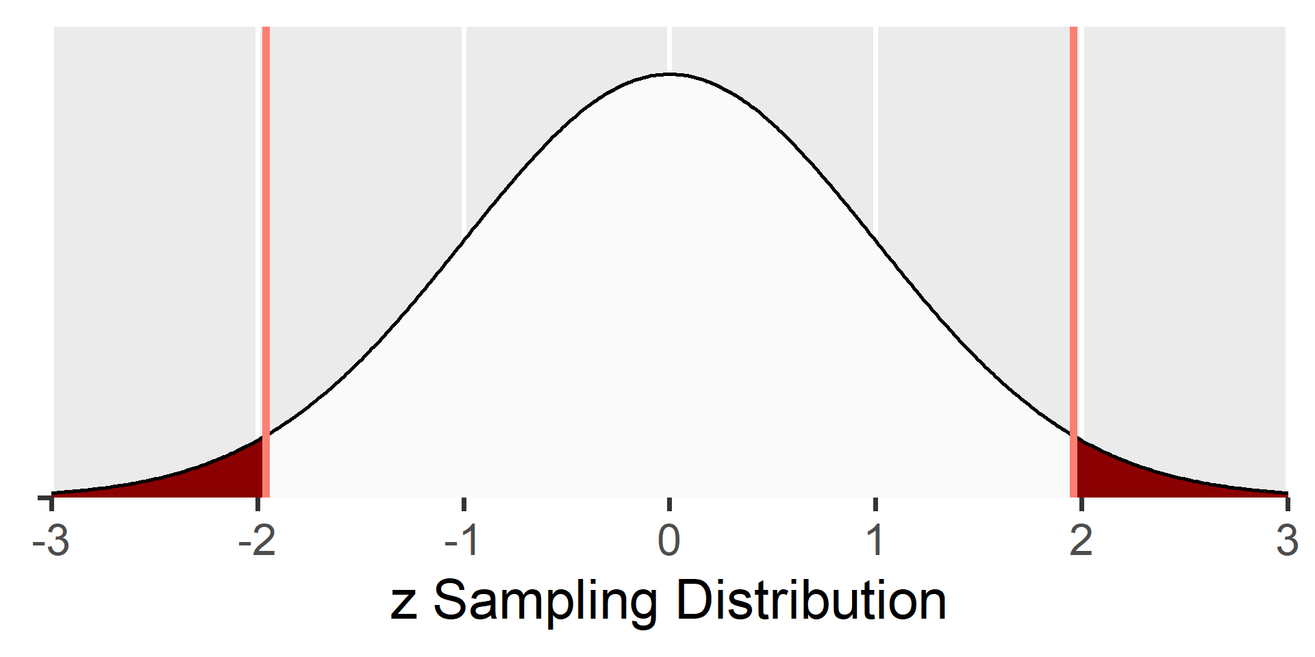
Single sample z-test
To set \alpha=.05, we reject the null if the test statistic is outside the middle 95% of its null sampling distribution
The math becomes easier if we standardize the test statistic by dividing it by its standard error
z_{\bar{x}} = \frac{\bar{x} - \mu_0}{\sigma / \sqrt{n}} \\ z_{\bar{x}} \sim \mathcal{N}(0, 1)
Critical values: |z_{\bar{x}}| > 1.96 (i.e., it falls in the red regions)
Single sample t-test
This z-test is rarely used because \sigma is rarely known
Instead, we estimate \sigma using s and use the t-test
With a small sample, the critical values are now higher
t_{\bar{x}} = \frac{\bar{x} - \mu_0}{s / \sqrt{n}} \\ t_{\bar{x}} \sim t(n-1, 0, 1)
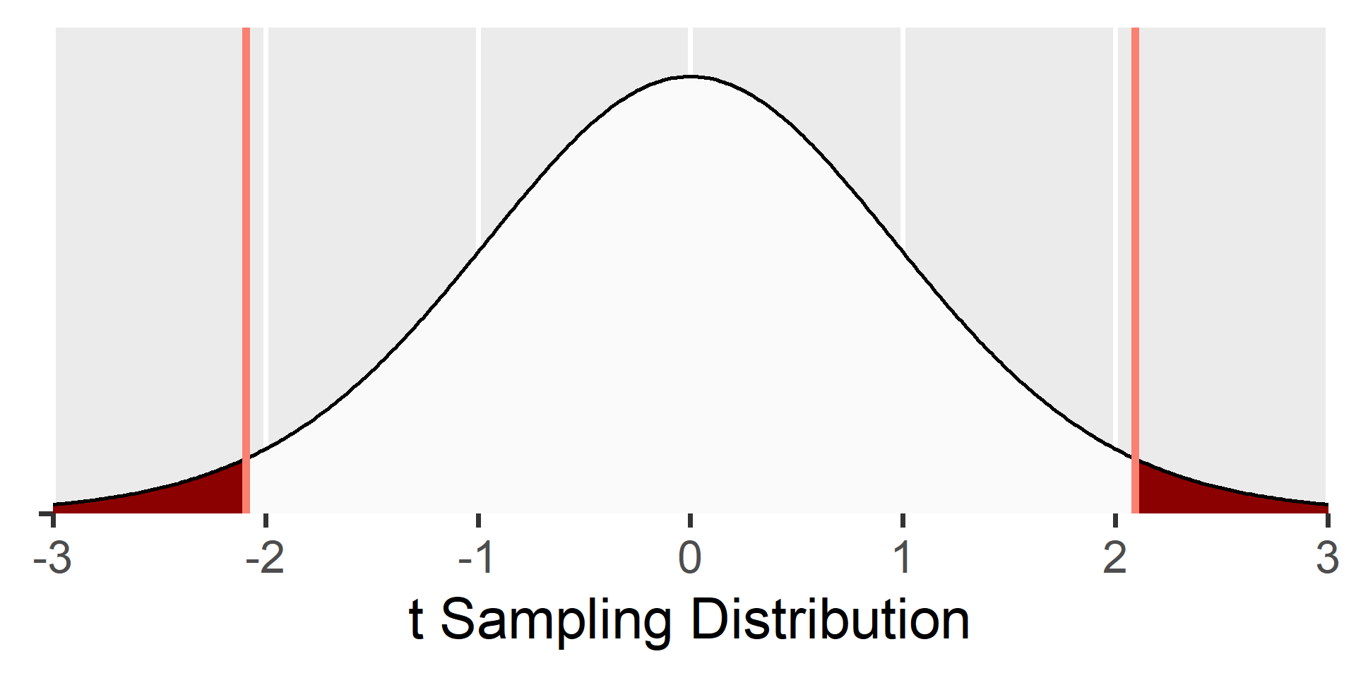
Critical values: |t_{\bar{x}}| > 2.09 (i.e., it falls in the red regions)
Example where H_0 is true
Imagine H_0 is true (\mu=3) and we collect the following sample of 20 cereal boxes
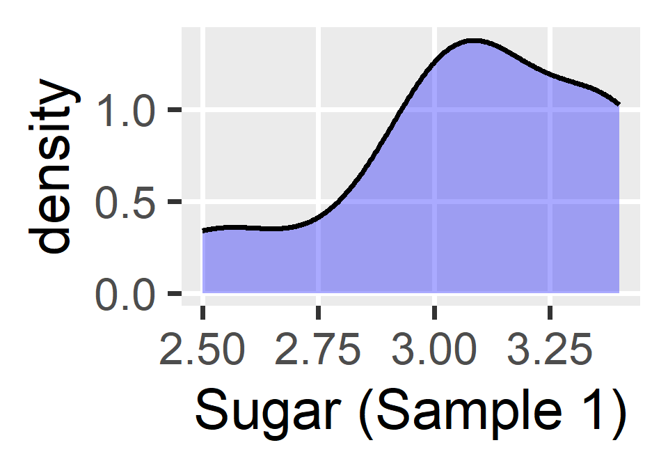
Example where H_0 is true
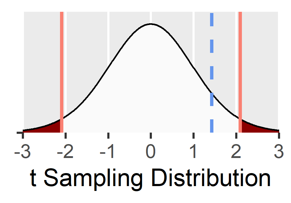
|t_{\bar{x}}|<t_{crit}: \text{Retain }H_0
Example where H_0 is false
Imagine H_0 is false (\mu=4) and we collect the following sample of 20 cereal boxes
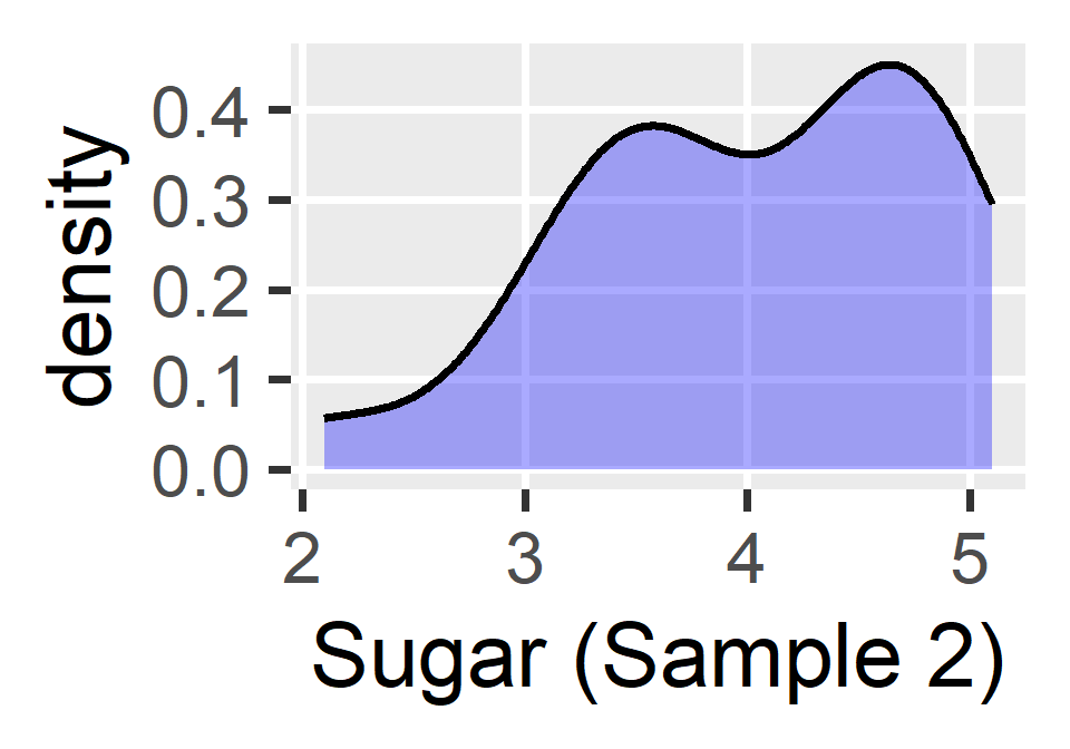
Example where H_0 is false
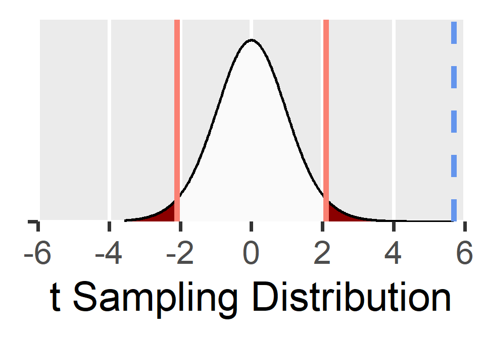
|t_{\bar{x}}|>t_{crit}: \text{Reject }H_0
Making decisions
- Critical values let us decide and control \alpha
- |t_{obs}| < t_{crit} = Retain the null
- |t_{obs}| \ge t_{crit} = Reject the null
- When we reject the null, the test was “significant”
- Remember that not all rejections are correct
- Even a correct rejection may not be important
- In a large sample, a small effect may be significant
p-values and
Pragmatics
The p-value of a test
- But what if we had selected a different \alpha level?
- Some \alpha values would yield a different decision
- The p-value is a popular approach for dealing with this
Correct p-value Definitions
The p-value is the smallest \alpha value that would reject the null hypothesis.
The p-value is the probability of observing a test statistic at least as extreme as ours, if the null hypothesis were true.
Wrong p-value Definition
The p-value is the probability that the null hypothesis is true.
Using the p-value
- The p-value is a summary of all possible \alpha values
- How would you feel about setting \alpha to p?
- It is best to set \alpha for the study before seeing the data
- Then, you reject the null if and only if p<\alpha
- Reporting p directly softens your decision
- e.g., p=.049 (Reject) vs. p=.051 (Retain)
- e.g., p=.002 (Reject) vs. p=.047 (Reject)
Reporting a significance test
| Notation | Stars | Translation | Decision |
|---|---|---|---|
| p ≥ .05 | Test was NOT significant at α=.05 | Retain Null | |
| p < .05 | * | Test was significant at α=.05 | REJECT Null |
| p < .01 | ** | Test was significant at α=.01 | REJECT Null |
| p < .001 | *** | Test was significant at α=.001 | REJECT Null |
- Report your exact p-value (unless less than .001)
- Saying p<.05 or p\ge.05 discards useful information
- It can be helpful to report a CI and your test statistic too
Putting it all together
- We can do a one-sample t-test in R with
t.test() - We can get a results table with
model_parameters()
fit1 <- t.test(sugar_null, mu = 3)

library(easystats)
model_parameters(fit1)
## One Sample t-test
##
## Parameter  | Mean | mu | Difference |       95% CI | t(19) |     p
## ------------------------------------------------------------------
## sugar_null | 3.09 |  3 |       0.09 | [2.96, 3.22] |  1.42 | 0.171
##
## Alternative hypothesis: true mean is not equal to 3
Interpreting the results
One Sample t-test

Parameter  | Mean | mu | Difference |       95% CI | t(19) |     p
------------------------------------------------------------------
sugar_null | 3.09 |  3 |       0.09 | [2.96, 3.22] |  1.42 | 0.171

Alternative hypothesis: true mean is not equal to 3
“The mean sugar content per serving in our sample was 3.09 g, 95% CI: [2.96, 3.22], which was not significantly different from the 3 g stated on the label, t(19)=1.42, p=.171. Thus, we retain the null hypothesis that there are 3 g of sugar per serving.”
Putting it all together… again
- Let’s repeat with the other sample
fit2 <- t.test(sugar_alt, mu = 3)

model_parameters(fit2)
## One Sample t-test
##
## Parameter | Mean | mu | Difference |       95% CI | t(19) |      p
## ------------------------------------------------------------------
## sugar_alt | 4.02 |  3 |       1.02 | [3.65, 4.39] |  5.70 | < .001
##
## Alternative hypothesis: true mean is not equal to 3
Interpreting the results
One Sample t-test

Parameter | Mean | mu | Difference |       95% CI | t(19) |      p
------------------------------------------------------------------
sugar_alt | 4.02 |  3 |       1.02 | [3.65, 4.39] |  5.70 | < .001

Alternative hypothesis: true mean is not equal to 3
“The mean sugar content per serving in our sample was 4.02 g, 95% CI: [3.65, 4.39], which was significantly greater than the 3 g stated on the label, t(19)=5.70, p<.001. Thus, we reject the null hypothesis that there are 3 g of sugar per serving.”