Statistical Methods with R

Confidence Intervals

Unit B · Chapter 04 · Lecture 04b

Developed by Jeffrey M. Girard

Types of Estimates

Point and Interval Estimates

In statistical inference, we will often want two types of estimates…

Point Estimates

  • What is our single best guess for the
    value of the population parameter?

  • This is usually the sample statistic

  • Does not say anything about uncertainty

e.g., I don’t know for sure the average height of all adult men, but I will guess that it is equal to the average height in my sample

Interval Estimates

  • What is a range of reasonable guesses for the value of the population parameter?

  • Usually the statistic plus/minus some amount that is based on uncertainty

e.g., Due to sampling error, any number within 2.9 cm of the average height in my sample is also a very reasonable guess

Reasonable values

  • Our uncertainty comes from the fact that sampling error causes different samples to yield different estimates

  • The sampling distribution shows what statistic values would be more or less common across many such samples

  • Reasonable values would be those where the sampling distribution is densest (i.e., the values that are the most commonly observed across different samples)

  • With less uncertainty (e.g., larger samples), the range of reasonable values will be tighter/narrower

Sampling distribution

  • But we don’t have access to the sampling distribution!
    • This is because we usually only take one sample…
  • So we will need to estimate the statistic values for which
    the sampling distribution is densest
    • There are many different techniques for doing this
  • We will use the frequentist parametric approach
    • This approach is very common and assumes that
      the sampling distribution is normally distributed
    • What does that mean? Is it reasonable to assume?

The Normal Distribution

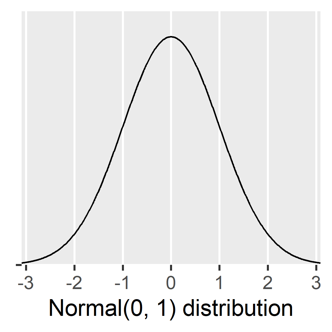
The normal distribution

The Normal Distribution is also called the Bell Curve and the Gaussian distribution

We say that \(x\) is normally distributed with mean \(\mu\) and standard deviation \(\sigma\) as

\[x \sim \text{Normal}(\mu, \sigma)\\x \sim \mathcal{N}(\mu,\sigma)\]

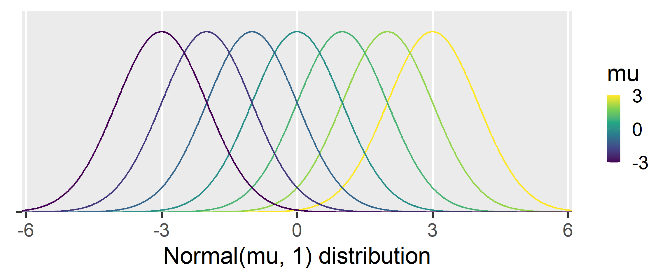
  • \(\mu\) (mu) determines the mean
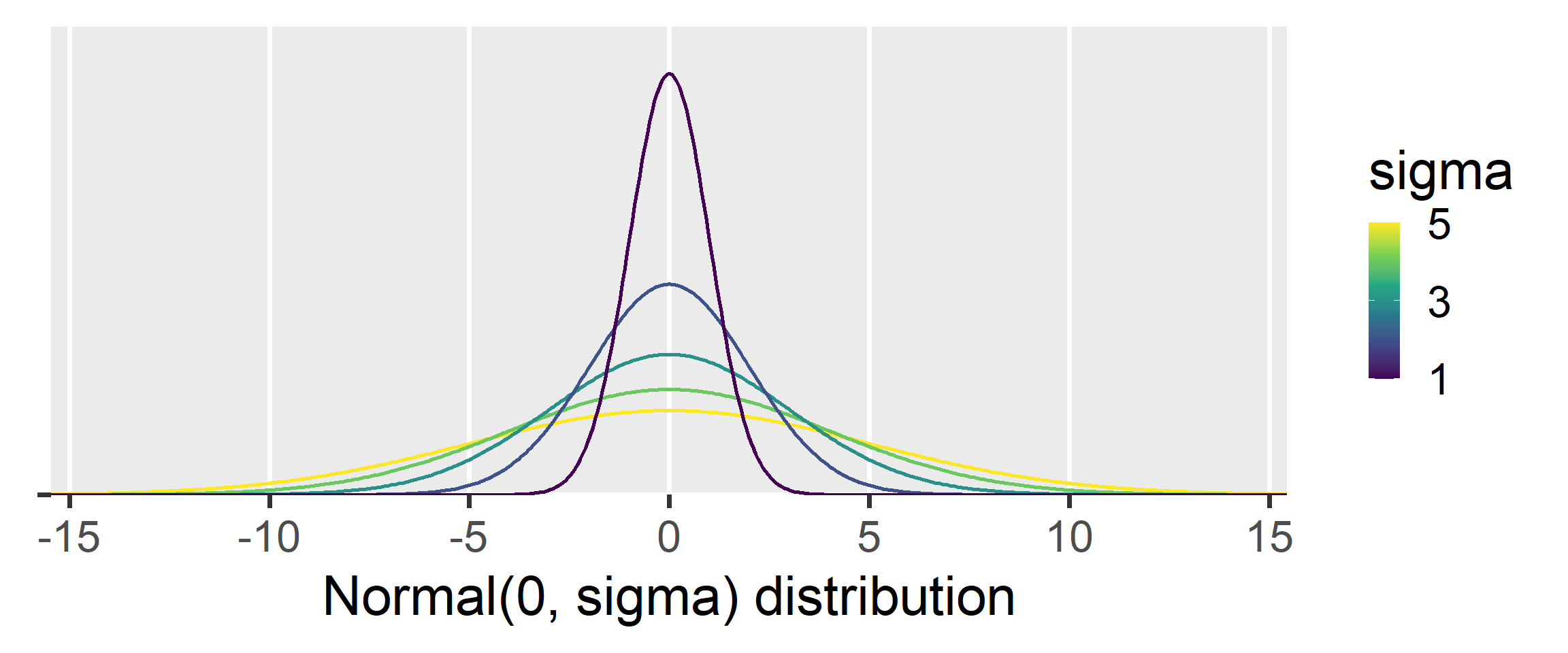
  • \(\sigma\) (sigma) determines the SD

The \(\mathcal{N}(0,1)\) distribution is called
the “Standard Normal Distribution”

The mu parameter

Changing \(\mu\) shifts the distribution left (\(-\)) or right (\(+\))

The sigma parameter

Changing \(\sigma\) expands (\(+\)) or contracts (\(-\)) the distribution

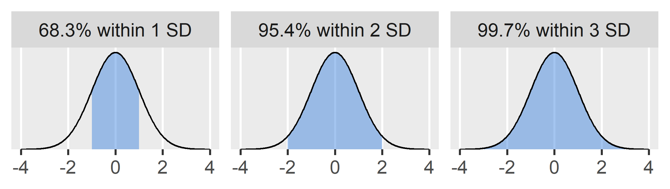
The empirical rule

~68.3% of the Normal distribution falls within 1 SD of the mean
~95.4% of the Normal distribution falls within 2 SD of the mean
~99.7% of the Normal distribution falls within 3 SD of the mean

Quantiles in R

How many SDs contain a given percentage?

  • We want the middle 95%, so we cut the 5% in half

  • We thus calculate the 2.5th and 97.5th percentiles

  • qnorm() does this for the Normal distribution

qnorm(0.025)
## [1] -1.959964
qnorm(0.975)
## [1] 1.959964
  • So 95% of the Normal distribution is within ~1.96 SDs

Putting it all together

  1. Our interval estimate should be the densest part of the sampling distribution

  2. 95% of the density of a normal distribution is within ~1.96 SD of the mean

  3. The SD of the sampling distribution is the standard error (SE) of the statistic

  4. So, if we assume the sampling distribution is normally distributed, then…

  5. Our interval estimate is the sample statistic plus/minus 1.96 * SE

\[\text{CI}_{95} = \bar{x} \pm (1.96 \times s_{\bar{x}})\]

This is called the 95% Confidence Interval (CI) and we’ll talk about it more soon

But this parametric approach all hinges on the assumption of normality (#4)…

Central Limit Theorem

Non-normally distributed data

What happens to the sampling distribution of \(\bar{x}\)
when \(x\) itself is not normally distributed?

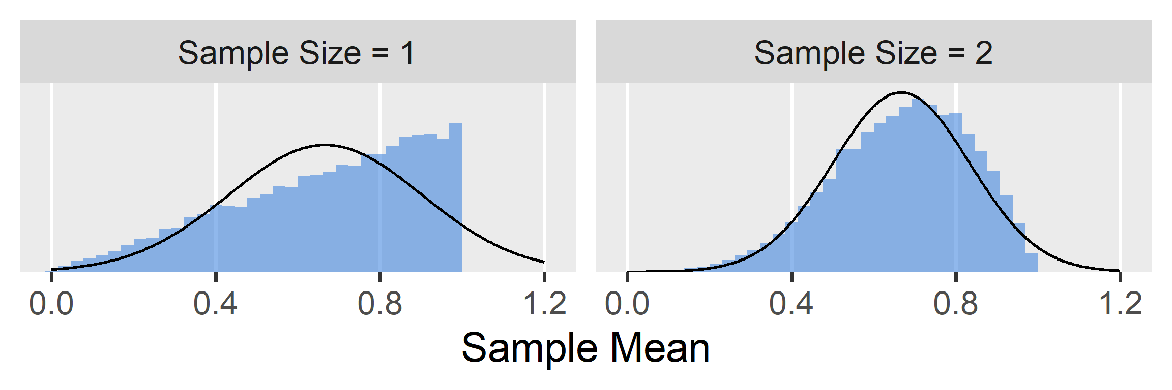
Central limit theorem

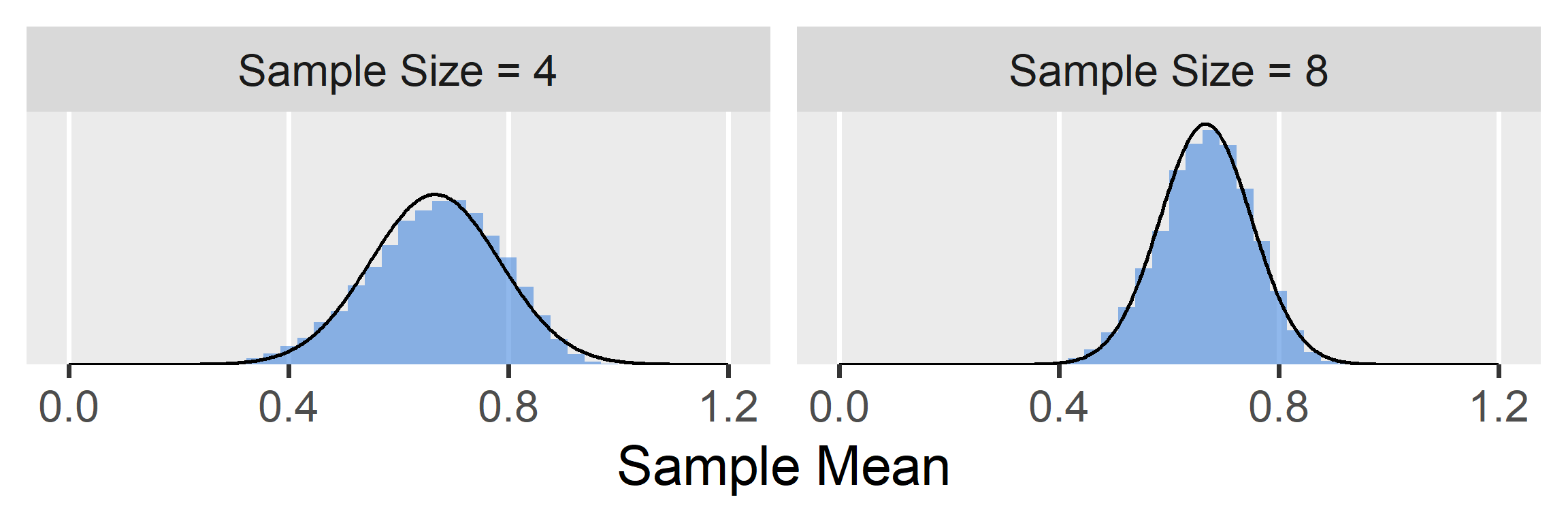
The sampling distribution of \(x\) will become more normal
as \(n\) increases (even if \(x\) itself is not normally distributed)

Normal approximations

  • The central limit theorem applies for almost all statistics
    • Why? Normal distributions come from summing up many random processes (e.g., genetic, environmental, social)
    • Some values will be higher and others will be lower
    • These deviations will tend to cancel each other out
    • Central values are common and extreme values are rarer
  • Thus, we often assume a normal sampling distribution…
    • This becomes more reasonable as \(n\) increases

Confidence Intervals

Calculations

  • To estimate the 95% Confidence Interval of the mean

\[\text{CI}_{95}= \bar{x}\pm\left(1.96\times\frac{\sigma}{\sqrt{n}}\right)\]

  • However, this requires that we know \(\sigma\), the population SD

  • Usually we estimate \(\sigma\) using \(s\), the sample SD

  • This estimation introduces a bit more uncertainty…

A complication

  • To account for this extra uncertainty, we need to…
    • Stop using the Normal distribution and qnorm()
    • Instead use the Student \(t\) distribution and qt()
  • The \(t\) distribution has more uncertainty when \(n\) is small
    • It becomes increasingly normal as \(n\) increases
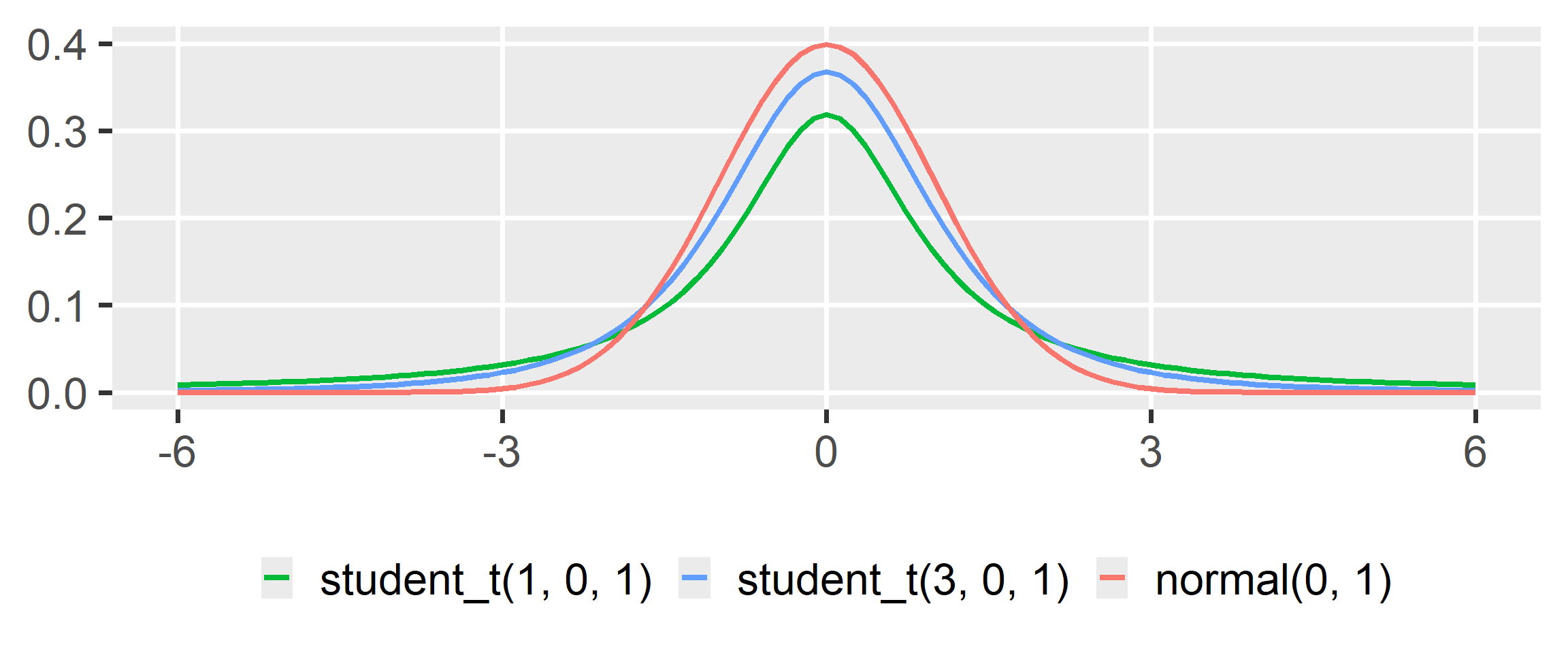
    • The \(t\) distribution has the same \(\mu\) and \(\sigma\) parameters
    • But it also has “degrees of freedom” \((\textit{df}=n-1)\)
    • As \(n\) increases, df increases, and \(t\) becomes more normal

The df parameter

As df increases, \(t(\textit{df},\mu,\sigma)\) becomes increasingly normal

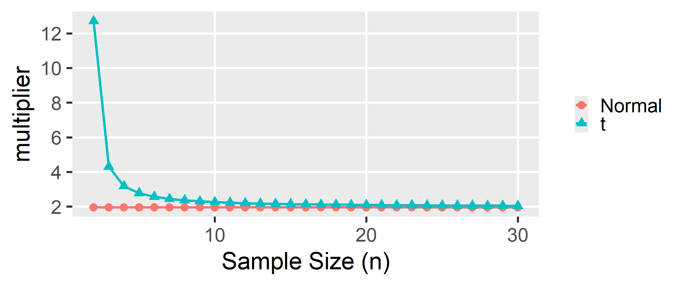
Comparing multipliers

When \(n\) is small, the \(t\) multiplier is higher (more uncertainty)

As \(n\) increases, the multipliers become increasingly similar
A correction to our formula

Population SD is known

\[\text{CI}_{\%}=\bar{x}\pm z \left(\frac{\sigma}{\sqrt{n}}\right)\]

# n = 20
(z <- qnorm(0.975))
## [1] 1.959964

# n = 100
(z <- qnorm(0.975))
## [1] 1.959964

Population SD is estimated

\[\text{CI}_{\%}=\bar{x}\pm t \left(\frac{s}{\sqrt{n}}\right)\]

# n = 20
(t <- qt(0.975, df = 20 - 1))
## [1] 2.093024

# n = 100
(t <- qt(0.975, df = 100 - 1))
## [1] 1.984217

An example in R

tratings <- read_csv("../../data/teaching_ratings.csv")
summary(tratings$eval)
##    Min. 1st Qu.  Median    Mean 3rd Qu.    Max. 
##   2.300   3.647   3.935   3.906   4.215   4.790

Estimate mean and SE

x <- tratings$eval
n <- length(x)
xbar <- mean(x)
s <- sd(x)
se <- s / sqrt(n)

xbar
## [1] 3.906064
se
## [1] 0.04753455

Estimate confidence interval

t <- qt(0.975, df = n - 1)
ci_lo <- xbar - (t * se)
ci_hi <- xbar + (t * se)

ci_lo
## [1] 3.81167
ci_hi
## [1] 4.000458

Practical Matters

Reporting a CI

  • It is recommended to always report point and interval estimates together

  • Reporting in text often uses this format:

    • Statistic = Point Estimate, X% CI: [Lower Bound, Upper Bound]
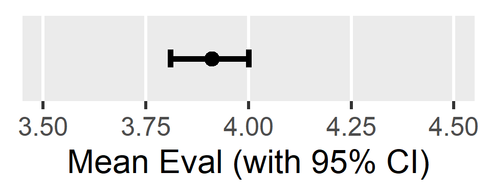
    • e.g., \(\bar{x}=3.91\), 95% CI: \([3.81, 4.00]\)
  • You can also put point and interval estimates in a table or a figure (though be sure to specify that they are X% CIs)

Example Table

Parameter Estimate 95% CI
Mean Eval 3.91 [3.81, 4.00]

Example Figure

Comparing CIs

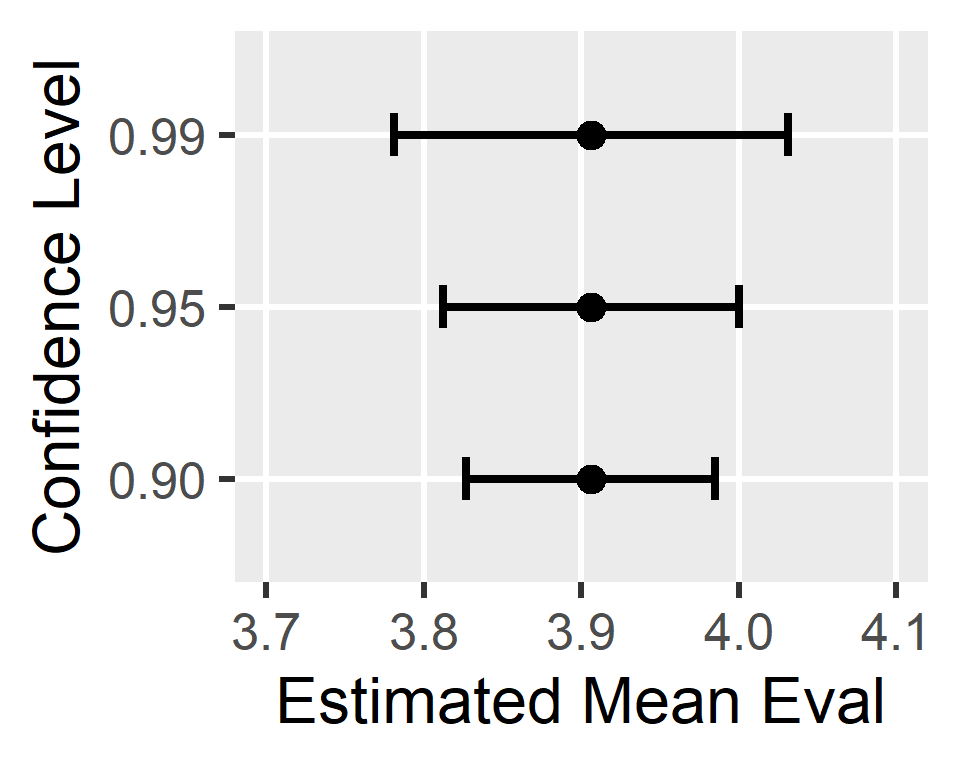
  • A higher confidence level will result in a wider interval
    • It is actually a riskier guess to be more confident
library(lsr)

ciMean(x, conf = 0.99)
##       0.5%    99.5%
## x 3.781061 4.031067

ciMean(x, conf = 0.95)
##      2.5%    97.5%
## x 3.81167 4.000458

ciMean(x, conf = 0.90)
##        5%      95%
## x 3.82709 3.985038

Interpreting CIs

It is common to misinterpret what confidence intervals mean

Incorrect Interpretation

“There is a 95% probability that the population parameter value lies within the 95% CI.”

The above is incorrect because it does not align with the frequentist view of probability

Interpreting CIs

The correct frequentist interpretation is quite a mouthful

Correct Interpretation

“If we repeated the experiment over and over again (with different samples of the same size) and computed the 95% CI in each sample, then 95% of those intervals would contain the population parameter value.”

Alternatives that are reasonable shortcuts

Acceptable Interpretations

“We can be 95% confident that the 95% CI contains the population mean.”

“The 95% CI contains highly reasonable estimates of the population mean.”

Another example

Let’s estimate the mean sleep satisfaction of all grad students

We have a sample of 16 grad students that we can use

sleep <- read_csv("../../data/sleep.csv")

mean(sleep$satisfaction)
## [1] 68.75

ciMean(sleep$satisfaction, conf = 0.95)
##          2.5%    97.5%
## [1,] 57.77683 79.72317

“We estimate that the mean sleep satisfaction among all grad students is 68.75, 95% CI: [57.78, 79.72]. Thus, our best guess for this value is 68.75 but, given sampling error, any number from 57.78 to 79.72 would also be a highly reasonable guess.”