# Read in data from file
library(tidyverse)
sleep <- read_csv("../../data/sleep.csv")
# Calculate total sleep hours
sleep$total <-
sleep$night + sleep$day
sleep$total [1] 8.0 6.0 7.5 9.0 9.0 8.0 6.0 8.0 7.0 9.0 8.0 9.0 6.0 7.5 7.0 7.0
Statistical Methods with R
Unit B · Chapter 04 · Lecture 04a
Developed by Jeffrey M. Girard
Uncertainty can be scary, uncomfortable, and dangerous
We strive to understand the world and make predictions
We often use our intuition and experiences to do so
We can do much better using the scientific method
See The Demon-Haunted World: Science as a Candle in the Dark by Sagan & Druyan
Start with a research question that is answerable with data
Generate a hypothesis (i.e., a testable prediction)
Conduct a replicable study to collect relevant data
Analyze the data to test the hypothesis/predictions
The scientific method classically uses experimental studies, but it can also improve observational studies
Question: Does caffeine make you smarter?
Hypothesis: Adult humans given caffeine will navigate a maze faster than adult humans not given caffeine.
Experiment: Recruit adult humans and give one group decaffeinated coffee and give another group normal coffee. Measure the time it takes each human to navigate a maze.
Analysis: Compare the two groups’ maze completion times.
Descriptive Statistics summarize and visualize the distributions and associations between variables
Inferential Statistics allow us to make inferences about our data and quantify the uncertainty in those inferences
Probability: Model \(\to\) Data
(e.g., given a fair coin, what is the chance of HHHHH…)
Statistics: Data \(\to\) Model
(e.g., given HHHHH, what is the chance the coin is fair…)
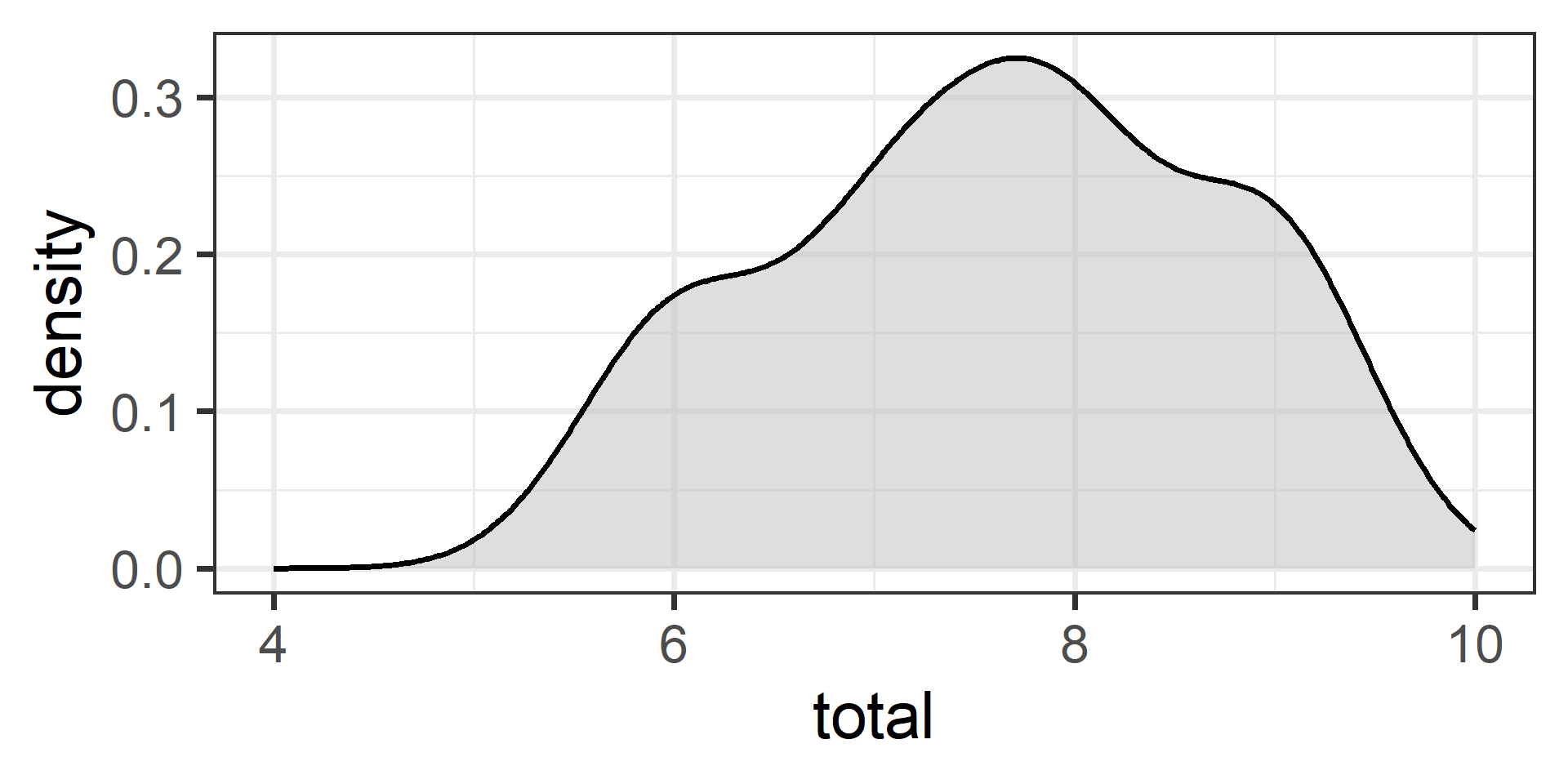
The population is the set of all possible observations that we want to draw conclusions and make predictions about
Imagine that we are interested in studying sleeping behavior
Are we interested in understanding the behavior of…
Populations aren’t always made up of people; you could have populations of groups, objects, events, etc.
A few years ago, I sent out a survey to every student in class
I was able to gather data for this entire population!
The mean represents the “typical” sleep duration
\[\mu=\frac{1}{N} \sum_{i=1}^N x_i\]
We denote parameters using Greek letters \((\mu,\sigma)\) or uppercase English letters \((N)\)
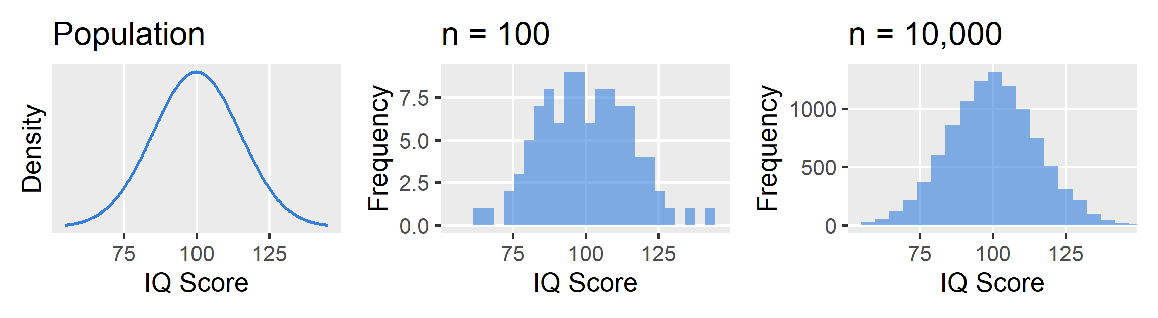
In practice, we are often interested in very large populations
It would be infeasible to measure such populations entirely
In these cases, we rely on sampling and statistical inference
A sample is a subset drawn from a population
Note we use lowercase \(n\) to denote the sample size
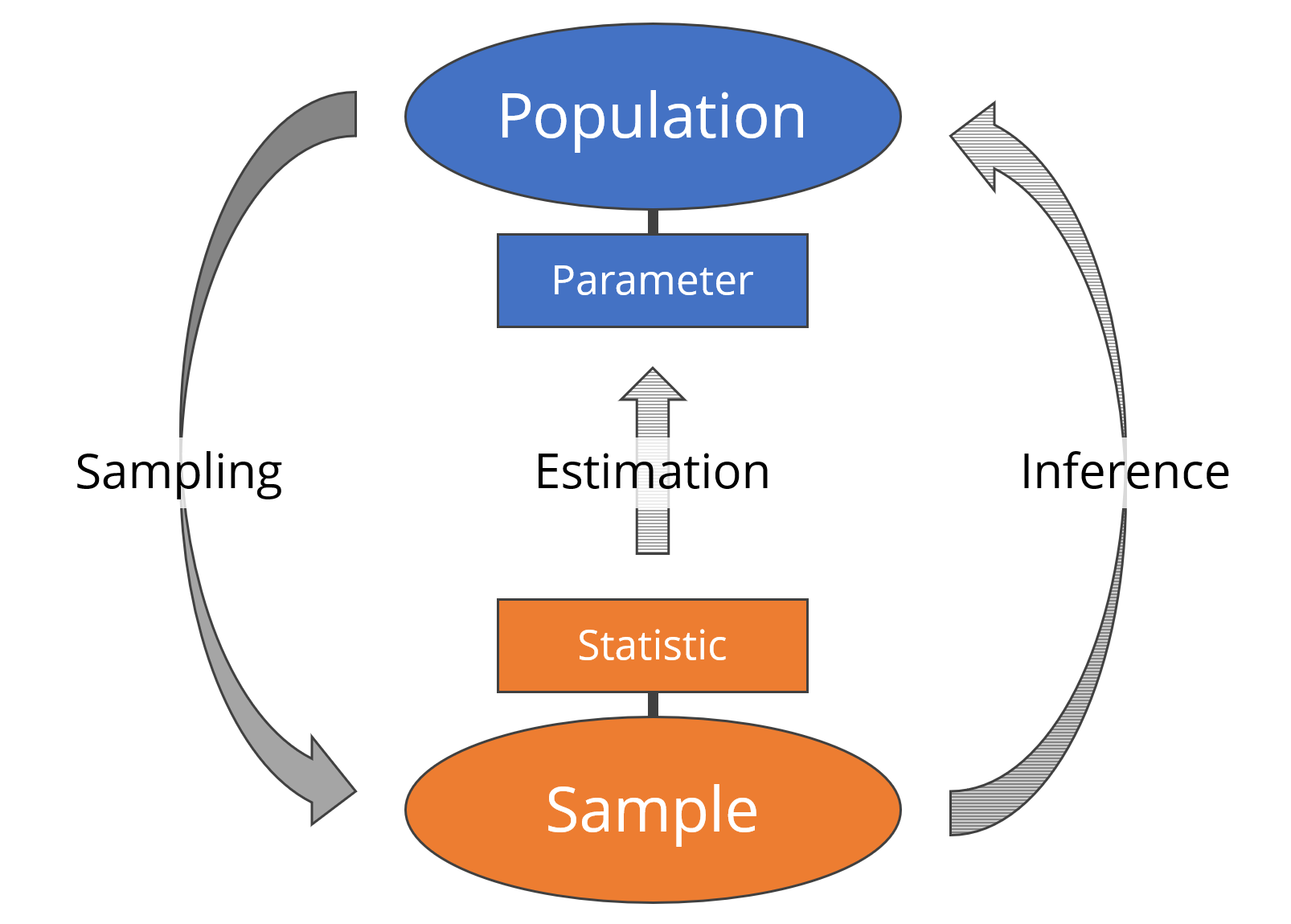
Sampling is drawing a subset of observations to represent a population
Inference is learning about the population by studying a sample drawn from it
We first measure in the sample whatever we want to know about the population
We call this measure the sample statistic
We use the sample statistic to estimate (i.e., guess) the population parameter

Our population is all the students in the class \((N=16)\) and our parameters of interest are the mean and SD of their total sleep time \((\mu=7.63, \sigma=1.04)\)
But imagine it is not feasible or possible to survey the entire population… so we randomly select six students to survey
In practice, we usually only have the sample’s data and so using sample() isn’t usually necessary
The mean formulas are basically identical for both samples and populations
\[\bar{x}=\frac{1}{n} \sum_{i=1}^n x_i\]
We denote sample statistics using lowercase English letters \((n, \bar{x},s)\) or Greek letters with hats \((\hat{\mu},\hat{\sigma})\)
Imagine we had drawn a sample of 2 instead of 6…
We might only sample part of the distribution
Now imagine we had drawn a sample of 14 instead of 6…
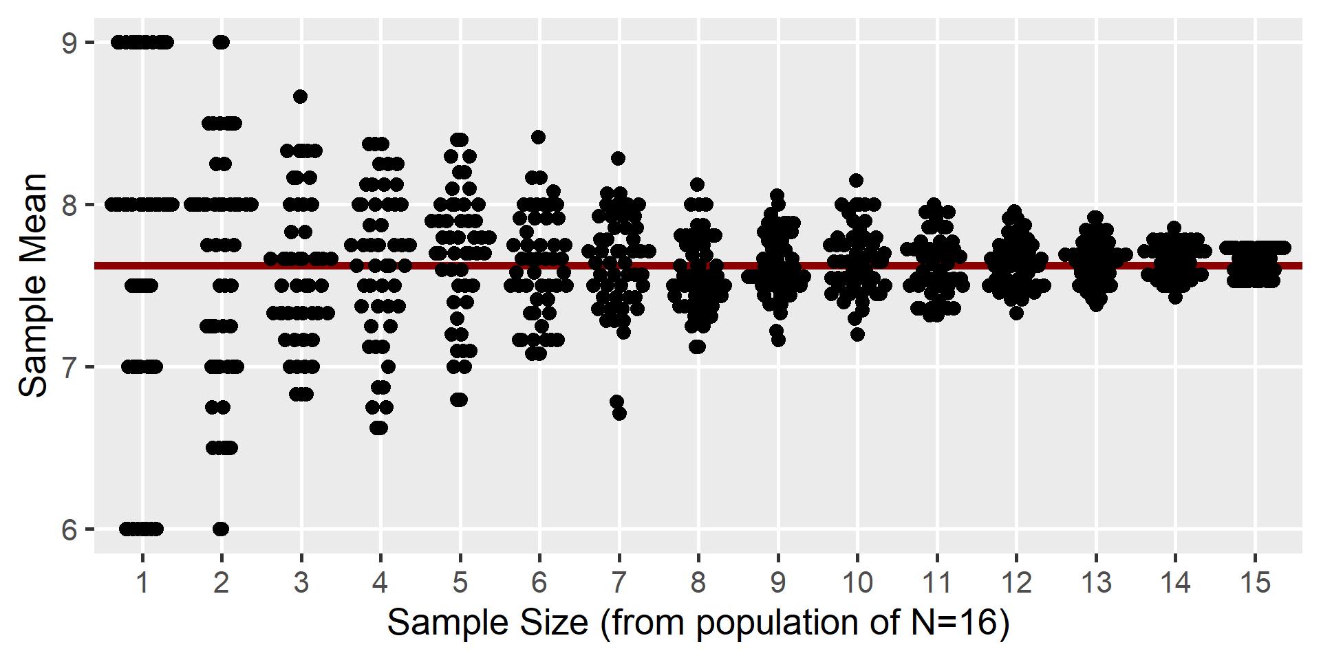
Larger (random) samples will tend to better approximate the population
Statistics from larger (random) samples will tend to better estimate the parameters
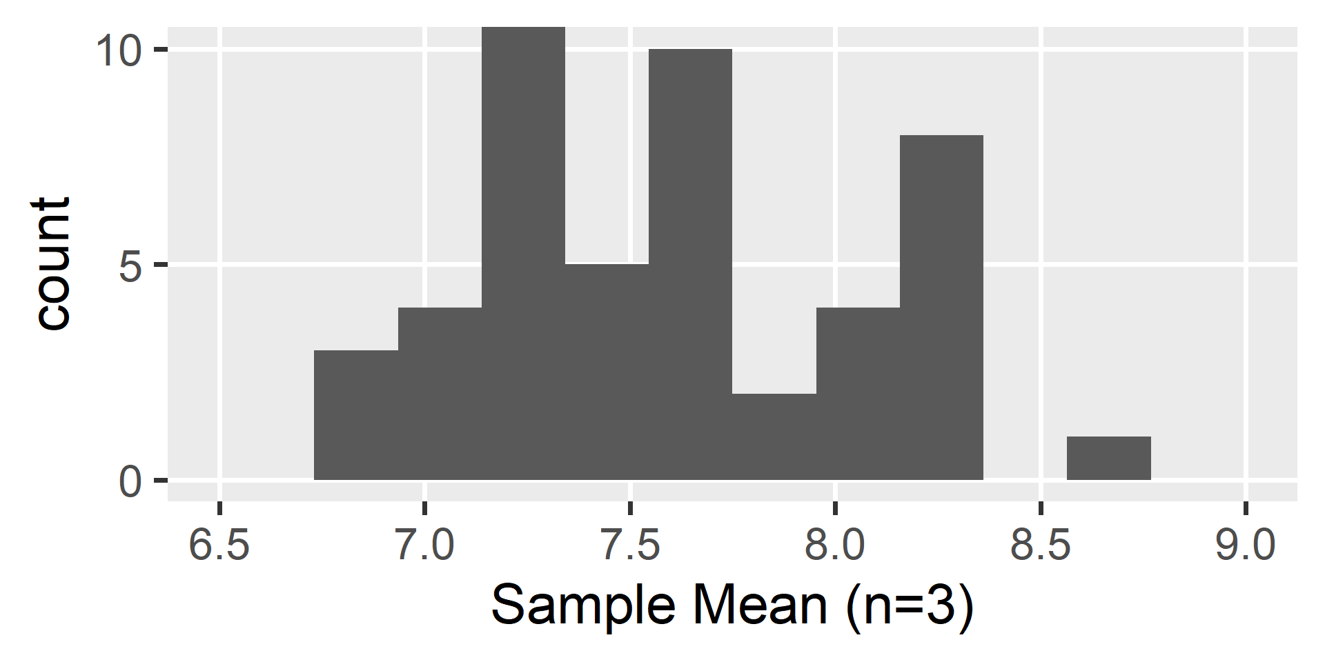
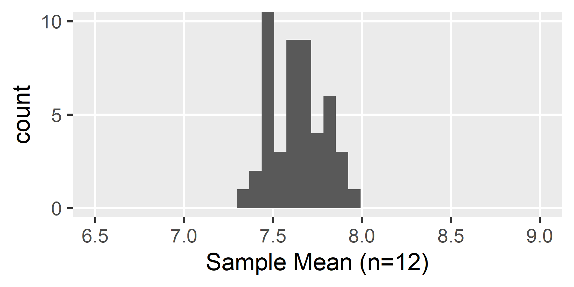
Let’s take samples of different sizes from our population and calculate the sample mean
To show the influence of chance, we can repeat this 50 times for each sample size
Let’s plot each repetition’s sample mean as a point (and the population mean as a line)
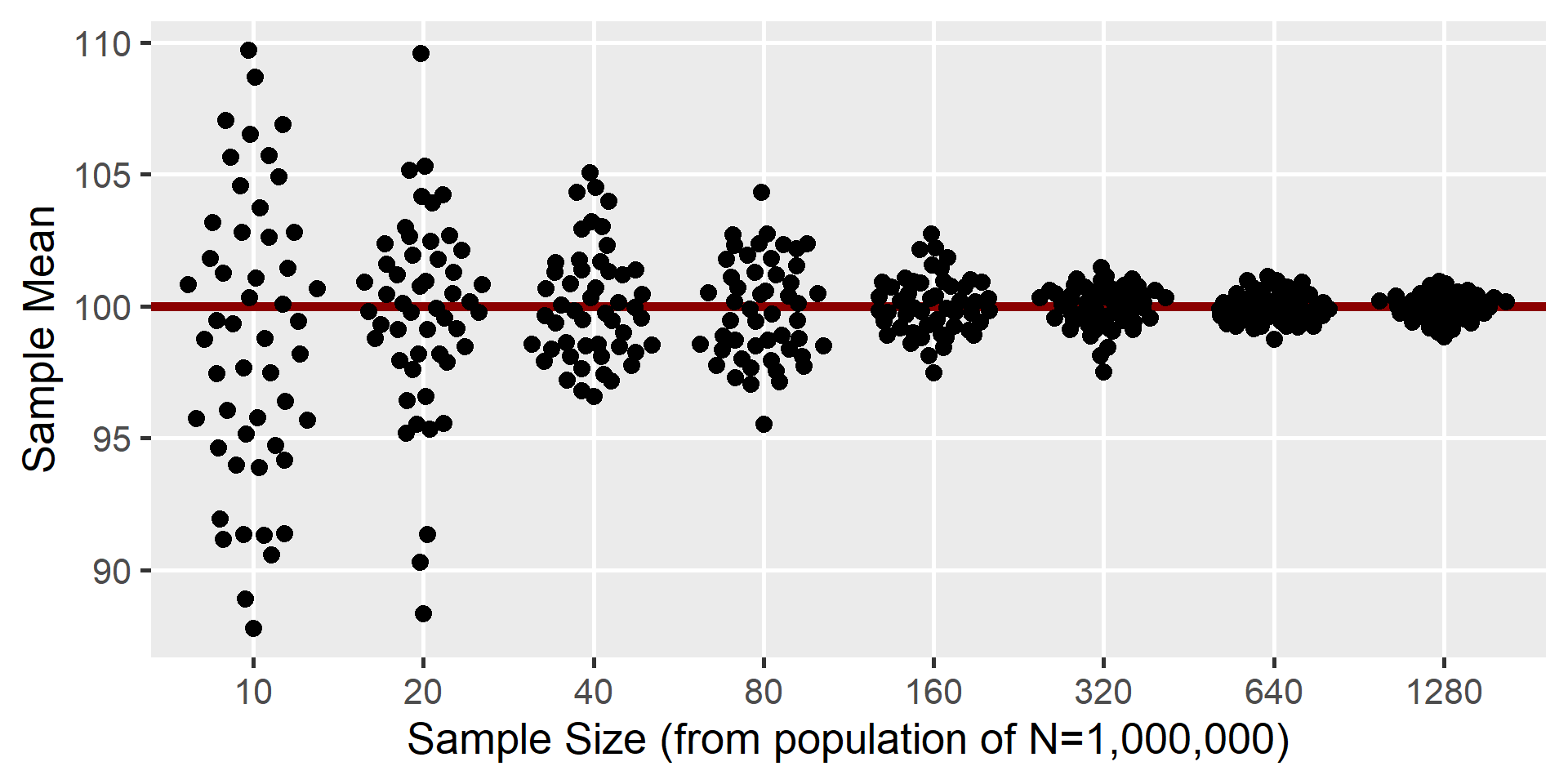
With larger populations, we need larger samples to get good estimates
Here is a simulation of sampling from a population \(N=1000000, \mu=100, \sigma=15\)
Repetitions of a study (with different samples) will result in different estimates due to sampling error
There is thus some uncertainty in our estimates/inferences due to sampling error
We can quantify the amount of sampling error in an estimate
Larger samples tend to decrease this uncertainty and “stabilize” our estimates (reducing sampling error)
However, larger populations require larger samples to achieve this benefit
The sampling distribution contains the statistic values from repeated samples
The wider the sampling distribution, the more uncertainty there is
The SD of the sampling distribution is called the standard error


We can rarely take many repeated samples, construct the sampling distribution, and calculate the SE directly
So, instead, we typically estimate the SE from the data (just like a parameter)
The estimate for the SE of the mean depends on two main things:
How large the sample is \((n)\)
How spread out the data is \((s)\)
\[s_{\bar{x}} = \frac{s}{\sqrt{n}} \sqrt{\frac{N-n}{N-1}}\]
As \(s\) increases, the SE increases
As \(n\) increases, the SE decreases
As \(n\to N\), the second part \(\to\) zero
As \(N\to\infty\), the second part \(\to\) one
Because we are often interested in infinite populations, the right side of this equation is often left off entirely.
The larger sample thus has a smaller estimated SE