These activities are for practice only; there is nothing to turn in. Answer keys are included, so try each question yourself before opening them.
Question 1
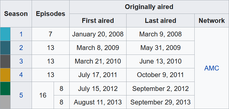
The following table summarizes the season information for the five seasons of AMC’s Breaking Bad show (the last split into two parts).
Tidy up this data and save it to a tibble. Decide for yourself how to handle season 5 (should it be a single observation or two?). For the first and last aired dates, just store the year as a number.
Save the tibble you created to a CSV file named “breaking_bad.csv”.
Answer key
Part (a)
Version with one observation for the season five parts
library (tidyverse)<- c (1 , 2 , 3 , 4 , 5 )<- c (7 , 13 , 13 , 13 , 16 )<- c (2008 , 2009 , 2010 , 2011 , 2012 )<- c (2008 , 2009 , 2010 , 2011 , 2013 )<- "AMC" <- tibble (season, episodes, first_air, last_air, network)
# A tibble: 5 × 5
  season episodes first_air last_air network
   <dbl>    <dbl>     <dbl>    <dbl> <chr>
1      1        7      2008     2008 AMC
2      2       13      2009     2009 AMC
3      3       13      2010     2010 AMC
4      4       13      2011     2011 AMC
5      5       16      2012     2013 AMC
Version with two separate observations for the season five parts
library (tidyverse)<- c (1 , 2 , 3 , 4 , 5.1 , 5.2 )<- c (7 , 13 , 13 , 13 , 8 , 8 )<- c (2008 , 2009 , 2010 , 2011 , 2012 , 2013 )<- c (2008 , 2009 , 2010 , 2011 , 2012 , 2013 )<- "AMC" <- tibble (season, episodes, first_air, last_air, network)
# A tibble: 6 × 5
  season episodes first_air last_air network
   <dbl>    <dbl>     <dbl>    <dbl> <chr>
1    1          7      2008     2008 AMC
2    2         13      2009     2009 AMC
3    3         13      2010     2010 AMC
4    4         13      2011     2011 AMC
5    5.1        8      2012     2012 AMC
6    5.2        8      2013     2013 AMC
Part (b)
write_csv (breaking_bad, "breaking_bad.csv" )
Question 2
Download the cereal.csv
Use {tidyverse} to import this file into R as a tibble named cereal, using an argument to make the missing values (coded as "missing") into NAs.
Run your command again but with the show_col_types = FALSE argument to suppress the column specification message.
Answer key
Part (b)
<- read_csv ("cereal.csv" , na = "missing" )
Rows: 77 Columns: 8
── Column specification ────────────────────────────────────────────────────────
Delimiter: ","
chr (3): name, mfr, type
dbl (5): calories, sodium, carbo, sugars, rating

ℹ Use `spec()` to retrieve the full column specification for this data.
ℹ Specify the column types or set `show_col_types = FALSE` to quiet this message.
# A tibble: 77 × 8
   name                      mfr       type  calories sodium carbo sugars rating
   <chr>                     <chr>     <chr>    <dbl>  <dbl> <dbl>  <dbl>  <dbl>
 1 100% Bran                 Nabisco   cold        70    130   5        6   68.4
 2 100% Natural Bran         Quaker O… cold       120     15   8        8   34.0
 3 All-Bran                  Kelloggs  cold        70    260   7        5   59.4
 4 All-Bran with Extra Fiber Kelloggs  cold        50    140   8        0   93.7
 5 Almond Delight            Ralston … cold       110    200  14        8   34.4
 6 Apple Cinnamon Cheerios   General … cold       110    180  10.5     10   29.5
 7 Apple Jacks               Kelloggs  cold       110    125  11       14   33.2
 8 Basic 4                   General … cold       130    210  18        8   37.0
 9 Bran Chex                 Ralston … cold        90    200  15        6   49.1
10 Bran Flakes               Post      cold        90    210  13        5   53.3
# ℹ 67 more rows
<- read_csv ("cereal.csv" , na = "missing" , show_col_types = FALSE )
Question 3
Update the cereal tibble from Question 2 to make the type variable a factor.
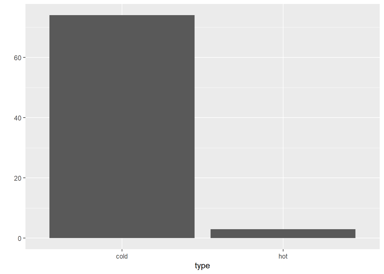
Tabulate the type variable using data_tabulate() and plot its discrete distribution using qplot().
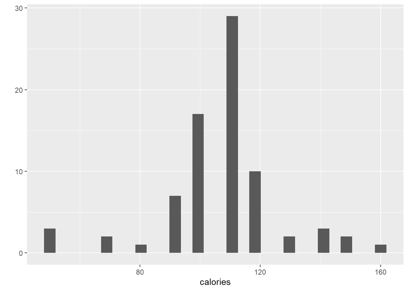
Describe the calories variable using describe_distribution() and plot its continuous distribution using qplot() and a “histogram” or “boxplot” geom.
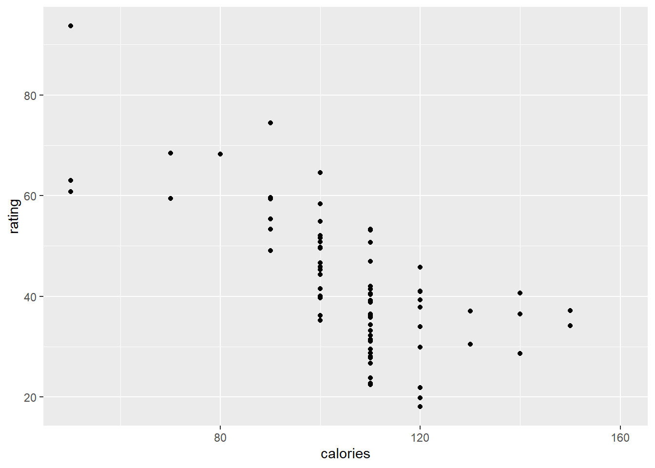
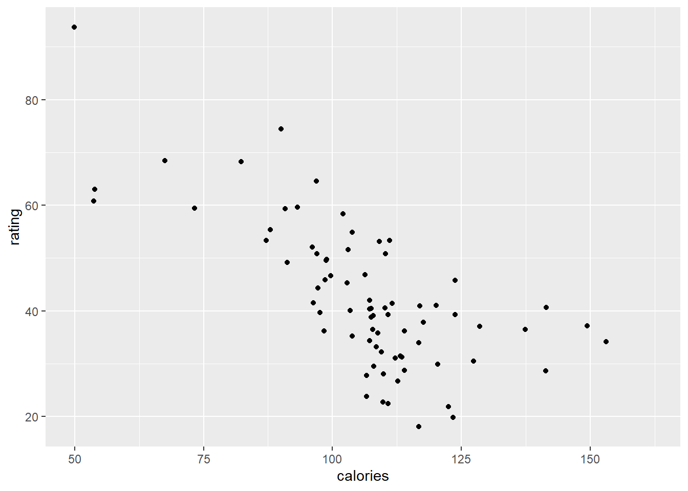
Plot the covariation of the calories and rating variables using qplot() and a “point” or “jitter” geom.
Answer key
Part (a)
$ type <- factor (cereal$ type)
# A tibble: 77 × 8
   name                      mfr       type  calories sodium carbo sugars rating
   <chr>                     <chr>     <fct>    <dbl>  <dbl> <dbl>  <dbl>  <dbl>
 1 100% Bran                 Nabisco   cold        70    130   5        6   68.4
 2 100% Natural Bran         Quaker O… cold       120     15   8        8   34.0
 3 All-Bran                  Kelloggs  cold        70    260   7        5   59.4
 4 All-Bran with Extra Fiber Kelloggs  cold        50    140   8        0   93.7
 5 Almond Delight            Ralston … cold       110    200  14        8   34.4
 6 Apple Cinnamon Cheerios   General … cold       110    180  10.5     10   29.5
 7 Apple Jacks               Kelloggs  cold       110    125  11       14   33.2
 8 Basic 4                   General … cold       130    210  18        8   37.0
 9 Bran Chex                 Ralston … cold        90    200  15        6   49.1
10 Bran Flakes               Post      cold        90    210  13        5   53.3
# ℹ 67 more rows
Part (b)
# Attaching packages: easystats 0.7.6
✔ bayestestR  0.18.1   ✔ correlation 0.8.8
✔ datawizard  1.3.1    ✔ effectsize  1.0.3
✔ insight     1.5.2    ✔ modelbased  0.16.0
✔ performance 0.17.1   ✔ parameters  0.29.2
✔ report      0.6.4    ✔ see         0.14.1
data_tabulate (cereal, type)
type (type) <categorical>
# total N=77 valid N=77

Value |  N | Raw % | Valid % | Cumulative %
------+----+-------+---------+-------------
cold  | 74 | 96.10 |   96.10 |        96.10
hot   |  3 |  3.90 |    3.90 |       100.00
<NA>  |  0 |  0.00 |    <NA> |         <NA>
qplot (x = type, data = cereal, geom = "bar" )
Warning: `qplot()` was deprecated in ggplot2 3.4.0.
Part (c)
describe_distribution (cereal, calories)
Variable |   Mean |    SD | IQR |           Range | Skewness | Kurtosis |  n | n_Missing
----------------------------------------------------------------------------------------
calories | 106.88 | 19.48 |  10 | [50.00, 160.00] |    -0.45 |     2.37 | 77 |         0
qplot (x = calories, data = cereal, geom = "histogram" )
`stat_bin()` using `bins = 30`. Pick better value `binwidth`.
Part (d)
qplot (x = calories, y = rating, data = cereal, geom = "point" )
Warning: Removed 2 rows containing missing values or values outside the scale range
(`geom_point()`).
qplot (x = calories, y = rating, data = cereal, geom = "jitter" )
Warning: Removed 2 rows containing missing values or values outside the scale range
(`geom_point()`).