Statistical Methods with R

Importing & Exploring

Unit A · Chapter 03 · Lecture 03b

Developed by Jeffrey M. Girard

Roadmap: More Programming

1. Data Frames

2. Data Files

3. Data Exploration

Data Frames

Tidy Data

• There are many ways to store data

• We will be learning the tidy data format
  • Data should be rectangular
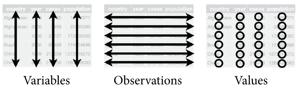
  • Each variable has its own column
  • Each observation has its own row
  • Each value has its own cell

Other Data Advice

• Name all variables in the first row
  • This is called a header row

• Avoid merged cells for data storage
  • These are okay for communication

• Avoid empty cells whenever possible
  • Mark missing data as NA

• Avoid formatting-as-data for storage
  • e.g., non-redundant color-coding

Tidying Example 1

Not Tidy

Name	Ann	Bob	Cat	Dom
Age	13	10	11	11
Weight	56.4	46.8	41.3	43.3

❌ Here, each row is a variable and each column is an observation.

Tidy

Name	Age	Weight
Ann	13	56.4
Bob	10	46.8
Cat	11	41.3
Dom	11	43.3

✔️ Here, each column is a variable and each row is an observation.

Tidying Example 2

Not Tidy

Names:	Ann	Bob	Cat	Dom
Age	Weight
13	56.4
10	46.8
11	41.3
11	43.3

❌ Here, we have data that is not rectangular because the Names variable has its own row.

Tidy

Name	Age	Weight
Ann	13	56.4
Bob	10	46.8
Cat	11	41.3
Dom	11	43.3

✔️ Here, we have made the data rectangular by moving the Names variable to its own column.

Tidying Example 3

Not Tidy

country	year	cases / population
Afghanistan	1999	NA / 19987071
	2000	2666 / 20595360
Brazil	1999	37737 / 172006362
	2000	80488 / 174504898
China	1999	212258 / 1272915272
	2000	213766 / 1280428583

❌ Here, we have merged cells and two values stored in a single cell.

Tidy

country	year	cases	population
Afghanistan	1999	NA	19987071
Afghanistan	2000	2666	20595360
Brazil	1999	37737	172006362
Brazil	2000	80488	174504898
China	1999	212258	1272915272
China	2000	213766	1280428583

✔️ Here, the countries are un-merged and cases and population have their own columns.

Tibbles

• R works particularly well with tidy data

• We store tidy data in data frames or tibbles
  • Tibbles are just fancier data frames
    (i.e., they have a few extra features)

• Tibbles need the tidyverse package

• Tibbles are built from vectors
  • The vectors must have the same length
  • They can contain different types of data

Parallel Vectors

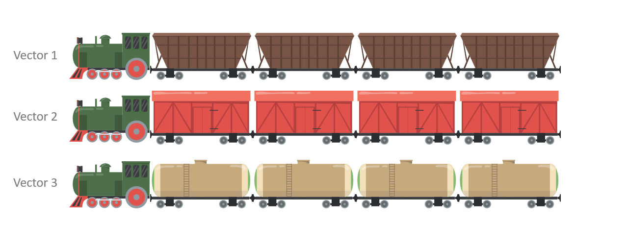
We start with three separate vector objects that all have the same length.

The n-th car in each train is the same observation.

Tibble

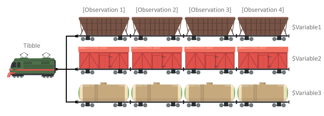
Then we combine the vectors into a single tibble (or data frame) object.

Now, as the tibble moves around, the variables always stay together.

This drawing is transposed. A train has to run lengthwise, so each variable is a row here. In a real tibble each variable is a column and each observation is a row, exactly as the tidy data rules said.

Loading the tidyverse

library(tidyverse)

── Attaching core tidyverse packages ──────────────────────── tidyverse 2.0.0 ──
✔ dplyr     1.2.1     ✔ readr     2.2.0
✔ forcats   1.0.1     ✔ stringr   1.6.0
✔ ggplot2   4.0.3     ✔ tibble    3.3.1
✔ lubridate 1.9.5     ✔ tidyr     1.3.2
✔ purrr     1.2.2     
── Conflicts ────────────────────────────────────────── tidyverse_conflicts() ──
✖ dplyr::filter() masks stats::filter()
✖ dplyr::lag()    masks stats::lag()
ℹ Use the conflicted package (<http://conflicted.r-lib.org/>) to force all conflicts to become errors

Install it once via Extras pane > Packages tab > Install, then load it each session. One library() call brings in the whole collection: readr, dplyr, ggplot2 and the rest. That is the only line most scripts need.

None of this is an error, even though RStudio prints it in red. The first block lists what got attached. Conflicts means two packages export the same name and dplyr won this round, so plain filter() now means dplyr’s. That is what you want here. Every later library(tidyverse) in these slides hides this message to save room.

A Tibble is Vectors Side by Side

x <- c(10, 20, 30, 40)

y <- x * 2 - 4
y

[1] 16 36 56 76

my_tibble <- tibble(x, y)
my_tibble

# A tibble: 4 × 2
      x     y
  <dbl> <dbl>
1    10    16
2    20    36
3    30    56
4    40    76

A column is a vector: tibble() stands them side by side, naming each column after its vector. That shape is what everything later assumes.

Tibbles Can Mix Types

first_names <- c("Adam", "Billy", "Caitlyn", "Debra")

age_years <- c(12, 13, 10, NA)

guests <- tibble(first_names, age_years)
guests

# A tibble: 4 × 2
  first_names age_years
  <chr>           <dbl>
1 Adam               12
2 Billy              13
3 Caitlyn            10
4 Debra              NA

Look at the <chr> and <dbl> labels: a tibble tracks each column’s type, and prints NA where a value is missing rather than guessing at one.

Pitfall: Unequal Column Lengths

tibble(y = c(1, 2, 3), x = c("a", "b"))

Error in `tibble()`:
! Tibble columns must have compatible sizes.
• Size 3: Existing data.
• Size 2: Column `x`.
ℹ Only values of size one are recycled.

Every column is one variable measured on the same rows, so they must all be the same length. R does make one exception: a column of length 1 is repeated down the whole tibble.

Extracting a Column with $

mytibble <- tibble(x = c(1, 2, 3, 4, 5), y = "test")

mytibble$x

[1] 1 2 3 4 5

mytibble$y

[1] "test" "test" "test" "test" "test"

$ pulls one column out as a plain vector. Note y: a single value is recycled down the column, because length one is the one length allowed to differ.

Pitfall: A Column That Does Not Exist

mytibble$z

Warning: Unknown or uninitialised column: `z`.

NULL

This is not an error. You get NULL and a warning, so a typo in a column name can flow silently into the rest of your code.

Getting Information About a Tibble

# Rows and columns
dim(guests)

[1] 4 2

# Column names
colnames(guests)

[1] "first_names" "age_years"  

Worth running on any dataset you did not build yourself, before you write code that assumes what is in it.

Data Files

Data Files

• Data is usually stored in data files
  • Importing files into R is called reading
  • Exporting files from R is called writing

• A convenient data file type is a CSV
  • This stands for comma-separated values
  • CSV files are easy to share

• The tidyverse package can read/write CSVs
  • Other packages read other types (readxl, haven, rio, googlesheets4)

Getting a Data File

• Download gradebook.csv from the course website into your project folder

• You can see it in the Extras pane > Files tab
  • And open it in another program, such as Excel

Reading in a Data File

old_gradebook <- read_csv("gradebook.csv")
old_gradebook

# A tibble: 3 × 2
     id grade
  <dbl> <chr>
1   123 95   
2   456 88   
3   789 ?    

read_csv() examines each column and guesses its type. You can state the types yourself, but the guess is usually right. Check it rather than assume it.

Pitfall: Missing Values in Disguise

old_gradebook <- read_csv("gradebook.csv", na = "?")
old_gradebook

# A tibble: 3 × 2
     id grade
  <dbl> <dbl>
1   123    95
2   456    88
3   789    NA

One grade was recorded as ?. R has no way to know that means “missing”. Until you say so with na = "?" it stays a real value, and the whole column is read as text rather than numbers.

Other Kinds of Data File

• readxl and googlesheets4: spreadsheets

• haven: files from SPSS, SAS, and STATA

• rio: tries to detect the type and read in anything

Data Exploration

Data Verification

• Always start with verification

• Check your variables are the correct type
  • Configure your factors’ levels and labels
  • Establish ordinal factors’ ordering
  • Explicitly set your missing values to NA

• Check variables’ extrema and distributions
  • Check for erroneous and outlying values
  • Check continuous variables’ shapes
  • Check the overlap of categorical levels

Reading in the Raw Penguins Data

library(easystats)

penguins <- read_csv("penguins0.csv")
penguins

# A tibble: 344 × 8
   species island bill_len bill_dep flipper_len body_mass   sex  year
     <dbl>  <dbl>    <dbl>    <dbl>       <dbl>     <dbl> <dbl> <dbl>
 1       1      3     39.1     18.7         181      3750     2  2007
 2       1      3     39.5     17.4         186      3800     1  2007
 3       1      3     40.3     18           195      3250     1  2007
 4       1      3     NA       NA            NA        NA    NA  2007
 5       1      3     36.7     19.3         193      3450     1  2007
 6       1      3     39.3     20.6         190      3650     2  2007
 7       1      3     38.9     17.8         181      3625     1  2007
 8       1      3     39.2     19.6         195      4675     2  2007
 9       1      3     34.1     18.1         193      3475    NA  2007
10       1      3     42       20.2         190      4250    NA  2007
# ℹ 334 more rows

species, island, and sex arrived as numbers, not categories.

Configuring the Factors

penguins$species <- factor(penguins$species, levels = c(1, 2, 3),
                           labels = c("Adelie", "Chinstrap", "Gentoo"))

penguins$island <- factor(penguins$island, levels = c(1, 2, 3),
                          labels = c("Biscoe", "Dream", "Torgersen"))

penguins$sex <- factor(penguins$sex, levels = c(1, 2),
                       labels = c("female", "male"))

The same factor() call as before, applied one column at a time with $. Tedious but explicit, and exactly the work a cleaning script exists to hold.

The Configured Data

penguins

# A tibble: 344 × 8
   species island    bill_len bill_dep flipper_len body_mass sex     year
   <fct>   <fct>        <dbl>    <dbl>       <dbl>     <dbl> <fct>  <dbl>
 1 Adelie  Torgersen     39.1     18.7         181      3750 male    2007
 2 Adelie  Torgersen     39.5     17.4         186      3800 female  2007
 3 Adelie  Torgersen     40.3     18           195      3250 female  2007
 4 Adelie  Torgersen     NA       NA            NA        NA <NA>    2007
 5 Adelie  Torgersen     36.7     19.3         193      3450 female  2007
 6 Adelie  Torgersen     39.3     20.6         190      3650 male    2007
 7 Adelie  Torgersen     38.9     17.8         181      3625 female  2007
 8 Adelie  Torgersen     39.2     19.6         195      4675 male    2007
 9 Adelie  Torgersen     34.1     18.1         193      3475 <NA>    2007
10 Adelie  Torgersen     42       20.2         190      4250 <NA>    2007
# ℹ 334 more rows

Those three columns now print as <fct> with readable values. Save the cleaned version with write_csv() so this is done once, not every session.

Checking the Summary for Problems

summary(penguins)

      species          island       bill_len        bill_dep    
 Adelie   :152   Biscoe   :168   Min.   :32.10   Min.   :13.10  
 Chinstrap: 68   Dream    :124   1st Qu.:39.23   1st Qu.:15.60  
 Gentoo   :124   Torgersen: 52   Median :44.45   Median :17.30  
                                 Mean   :43.92   Mean   :17.15  
                                 3rd Qu.:48.50   3rd Qu.:18.70  
                                 Max.   :59.60   Max.   :21.50  
                                 NAs    :2       NAs    :2      
  flipper_len      body_mass        sex           year     
 Min.   :172.0   Min.   :2700   female:165   Min.   :2007  
 1st Qu.:190.0   1st Qu.:3550   male  :168   1st Qu.:2007  
 Median :197.0   Median :4050   NAs   : 11   Median :2008  
 Mean   :200.9   Mean   :4202                Mean   :2008  
 3rd Qu.:213.0   3rd Qu.:4750                3rd Qu.:2009  
 Max.   :231.0   Max.   :6300                Max.   :2009  
 NAs    :2       NAs    :2                                 

Read the NA counts: 2 penguins were never measured and 11 (including those 2) were never sexed. Real data has holes, and this is where you find them.

Describing One Continuous Variable

describe_distribution(penguins, body_mass)

Variable  |    Mean |     SD |     IQR |              Range | Skewness
----------------------------------------------------------------------
body_mass | 4201.75 | 801.95 | 1206.25 | [2700.00, 6300.00] |     0.47

Variable  | Kurtosis |   n | n_Missing
--------------------------------------
body_mass |    -0.72 | 342 |         2

Mean, SD, range, and the count of missing values in one line: the numbers you would otherwise ask for one function at a time.

Describing All of Them at Once

describe_distribution(penguins)

Variable    |    Mean |     SD |     IQR |              Range | Skewness
------------------------------------------------------------------------
bill_len    |   43.92 |   5.46 |    9.30 |     [32.10, 59.60] |     0.05
bill_dep    |   17.15 |   1.97 |    3.12 |     [13.10, 21.50] |    -0.14
flipper_len |  200.92 |  14.06 |   23.25 |   [172.00, 231.00] |     0.35
body_mass   | 4201.75 | 801.95 | 1206.25 | [2700.00, 6300.00] |     0.47
year        | 2008.03 |   0.82 |    2.00 | [2007.00, 2009.00] |    -0.05

Variable    | Kurtosis |   n | n_Missing
----------------------------------------
bill_len    |    -0.88 | 342 |         2
bill_dep    |    -0.91 | 342 |         2
flipper_len |    -0.98 | 342 |         2
body_mass   |    -0.72 | 342 |         2
year        |    -1.50 | 344 |         0

Name no column and it describes every continuous one, skipping the factors. A good first look at a dataset you have just read in.

Tabulating One Factor

data_tabulate(penguins, species)

species (species) <categorical>
# total N=344 valid N=344

Value     |   N | Raw % | Valid % | Cumulative %
----------+-----+-------+---------+-------------
Adelie    | 152 | 44.19 |   44.19 |        44.19
Chinstrap |  68 | 19.77 |   19.77 |        63.95
Gentoo    | 124 | 36.05 |   36.05 |       100.00
<NA>      |   0 |  0.00 |    <NA> |         <NA>

The factor counterpart of describe_distribution(): counts and percentages, with missing values shown rather than dropped.

Tabulating Every Factor

data_tabulate(penguins, is.factor)

species (species) <categorical>
# total N=344 valid N=344

Value     |   N | Raw % | Valid % | Cumulative %
----------+-----+-------+---------+-------------
Adelie    | 152 | 44.19 |   44.19 |        44.19
Chinstrap |  68 | 19.77 |   19.77 |        63.95
Gentoo    | 124 | 36.05 |   36.05 |       100.00
<NA>      |   0 |  0.00 |    <NA> |         <NA>

island (island) <categorical>
# total N=344 valid N=344

Value     |   N | Raw % | Valid % | Cumulative %
----------+-----+-------+---------+-------------
Biscoe    | 168 | 48.84 |   48.84 |        48.84
Dream     | 124 | 36.05 |   36.05 |        84.88
Torgersen |  52 | 15.12 |   15.12 |       100.00
<NA>      |   0 |  0.00 |    <NA> |         <NA>

sex (sex) <categorical>
# total N=344 valid N=333

Value  |   N | Raw % | Valid % | Cumulative %
-------+-----+-------+---------+-------------
female | 165 | 47.97 |   49.55 |        49.55
male   | 168 | 48.84 |   50.45 |       100.00
<NA>   |  11 |  3.20 |    <NA> |         <NA>

Passing is.factor tabulates every factor at once: the categorical half of the same first look.

Data Visualization

• Variable distributions are critical in data analysis
  • What are the most and least common values?
  • What are the extrema (min and max values)?
  • Are there any outliers or impossible values?
  • How much spread is there in the variable?
  • What shape does the distribution take?

• Distributions describe a single variable’s variation
  • We also visualize many variables’ covariation

Loading the Cleaned Data

penguins <- read_csv("penguins.csv")

This is the tidied version of the file we just walked through: factors configured, missing values read correctly. Everything that follows uses it, and you will meet it again in later chapters.

Variation of a Factor

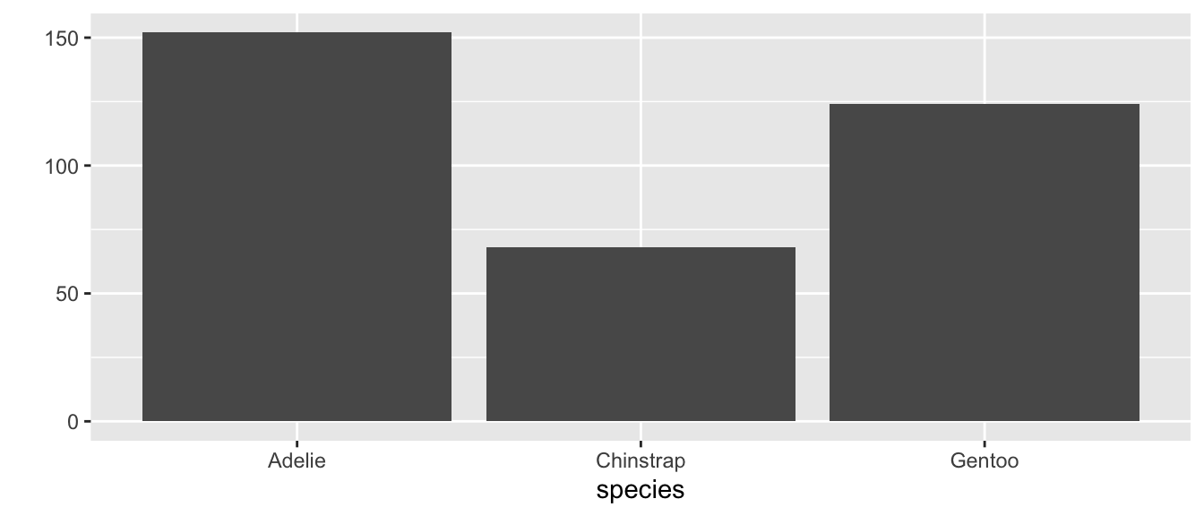
qplot(x = species, data = penguins, geom = "bar")

Warning: `qplot()` was deprecated in ggplot2 3.4.0.

Note. qplot() warns that it is deprecated. It still works and we will keep using it here; the warning appears once per session, not once per plot.

Variation of Another Factor

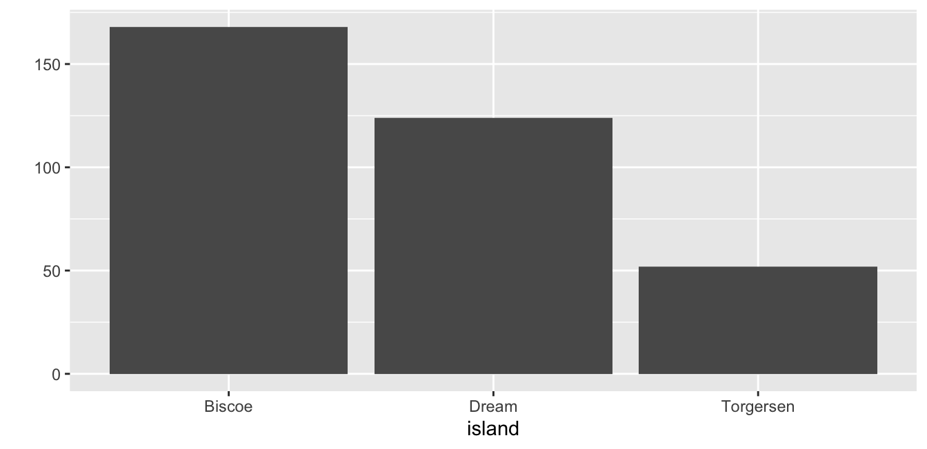
qplot(x = island, data = penguins, geom = "bar")

Variation of a Continuous Variable

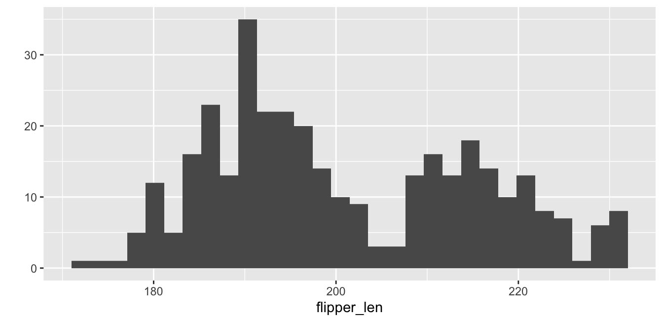
qplot(x = flipper_len, data = penguins, geom = "histogram")

The Same Variable as a Boxplot

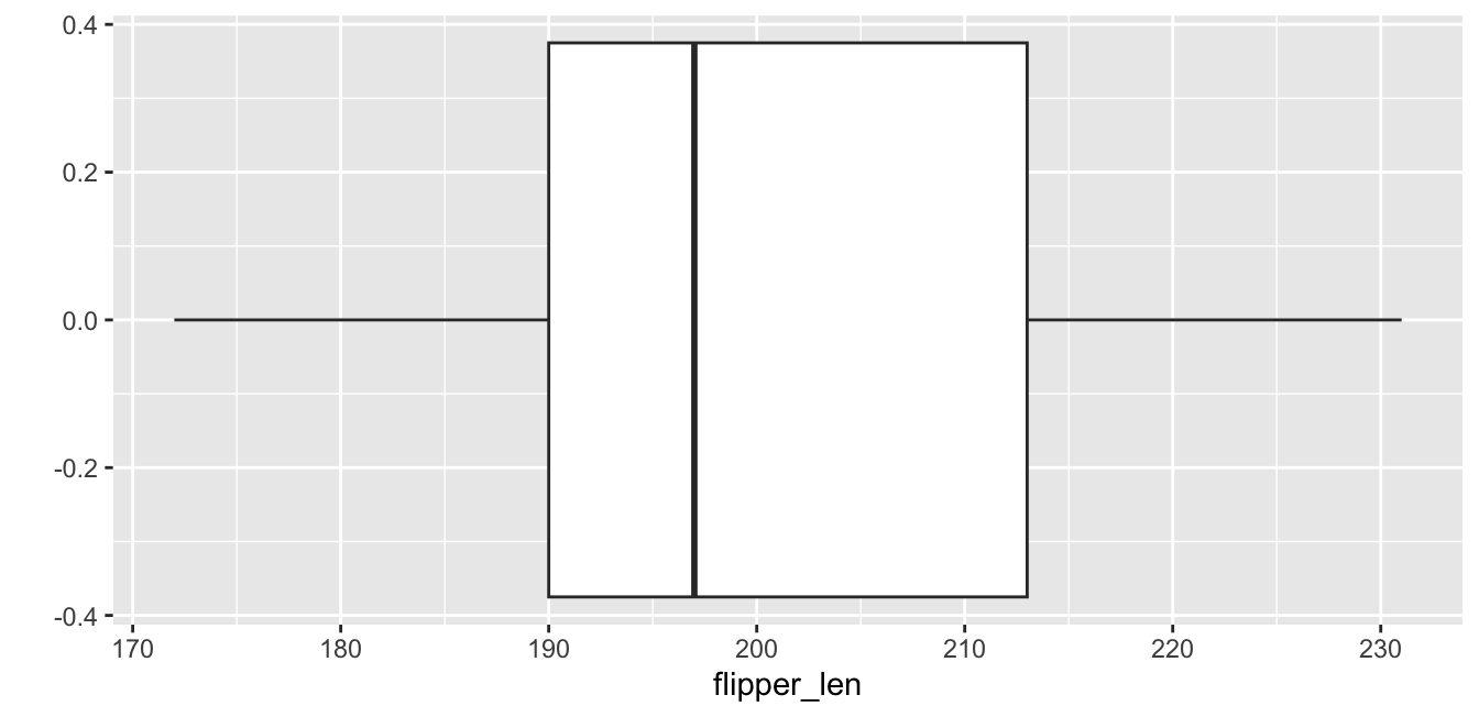
qplot(x = flipper_len, data = penguins, geom = "boxplot")

Body Mass as a Histogram

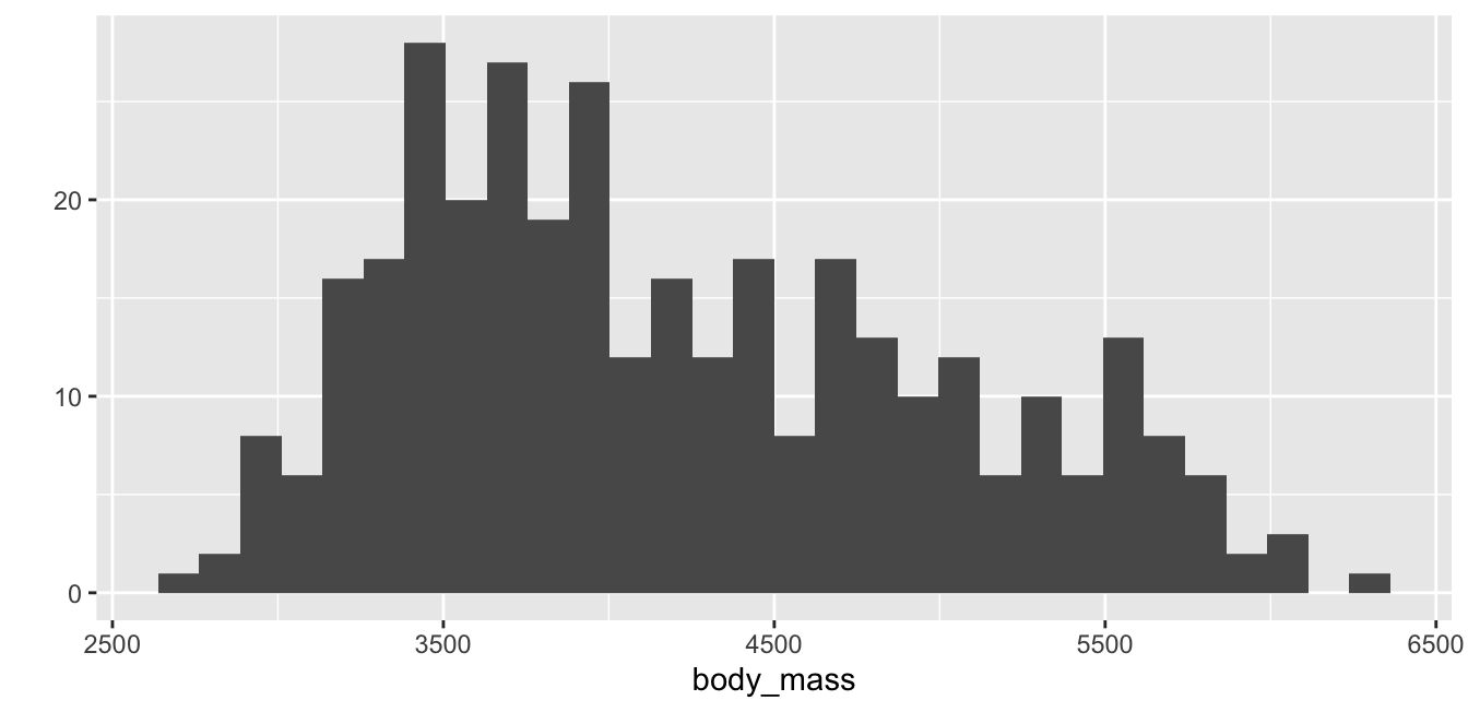
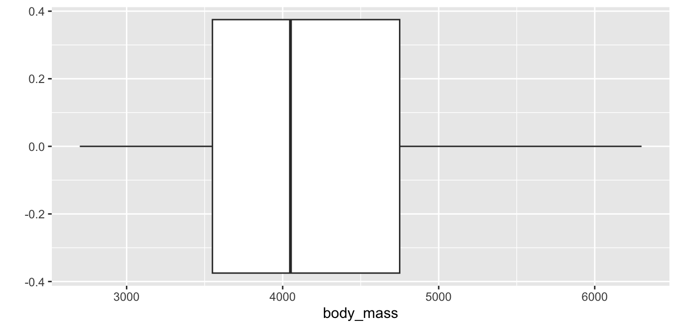
qplot(x = body_mass, data = penguins, geom = "histogram")

Body Mass as a Boxplot

qplot(x = body_mass, data = penguins, geom = "boxplot")

Two Continuous Variables

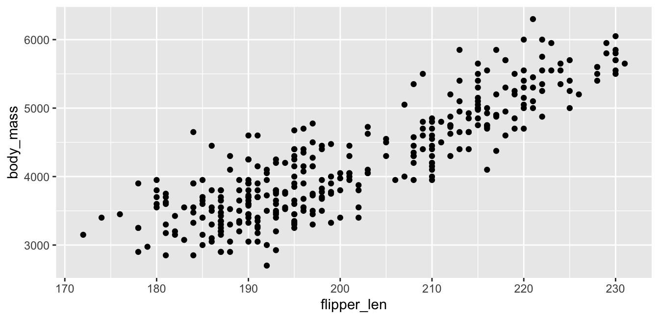
qplot(x = flipper_len, y = body_mass, data = penguins, geom = "point")

Covariation of Two Factors

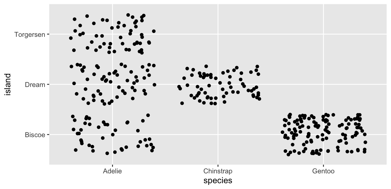
qplot(x = species, y = island, data = penguins, geom = "jitter")

The Same Pair as Stacked Bars

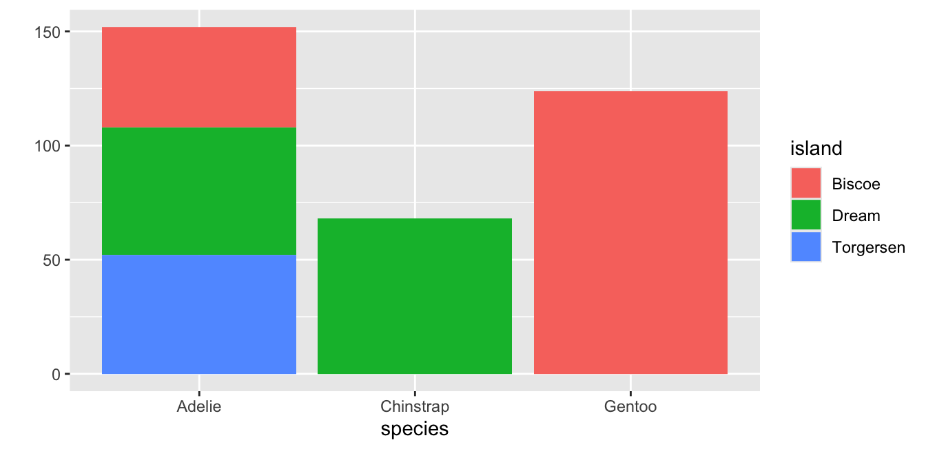
qplot(x = species, fill = island, data = penguins, geom = "bar")

A Factor and a Continuous Variable

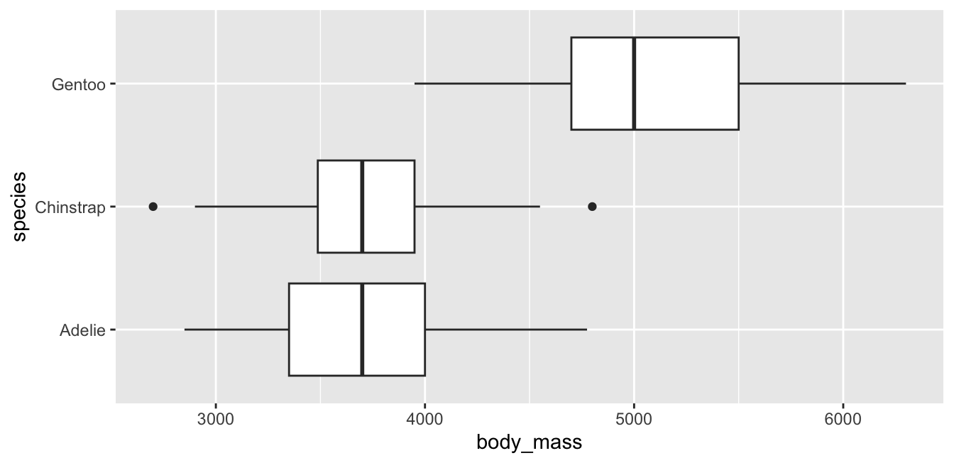
qplot(x = body_mass, y = species, data = penguins, geom = "boxplot")

The Same Pair as Violins

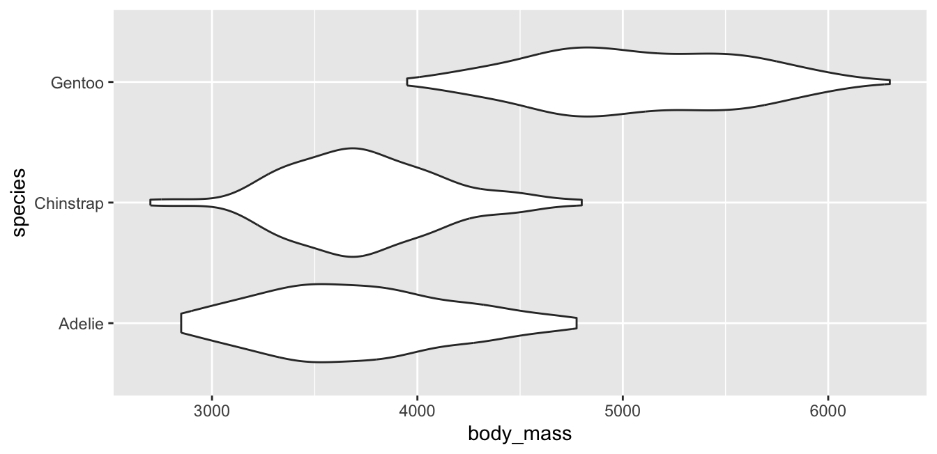
qplot(x = body_mass, y = species, data = penguins, geom = "violin")